Deep Learning
YOLOv5 PyTorch Tutorial
October 26, 2022
11 min read

YOLO, an acronym for 'You only look once,’ is an open-source software tool utilized for its efficient capability of detecting objects in a given image in real time. The YOLO algorithm uses convolutional neural network (CNN) models to detect objects in an image.
The algorithm requires only one forward propagation through a given neural network to detect all objects in the image. This gives the YOLO algorithm an edge in speed over others, making it one of the most well-known detection algorithms to date.
An object detection algorithm is an algorithm that is capable of detecting certain objects or shapes in a given frame. For example, simple detection algorithms may be capable of detecting and identifying shapes in an image such as circles or squares, while more advanced detection algorithms can detect more complex objects such as humans, bicycles, cars, etc.
Not only does the YOLO algorithm offer high detection speed and performance through its one-forward propagation capability, but it also detects them with great accuracy and precision.
In this tutorial, we will focus on YOLOv5, which is the fifth and latest version of the YOLO software. It was originally released on the 18th of May 2020. The YOLO open-source code can be found on GitHub. We will be using YOLO with the well-known PyTorch library.
PyTorch is a deep learning open-source package that is based on the well-known Torch library. It's also a Python-based library that is more commonly used for natural language processing and computer vision.
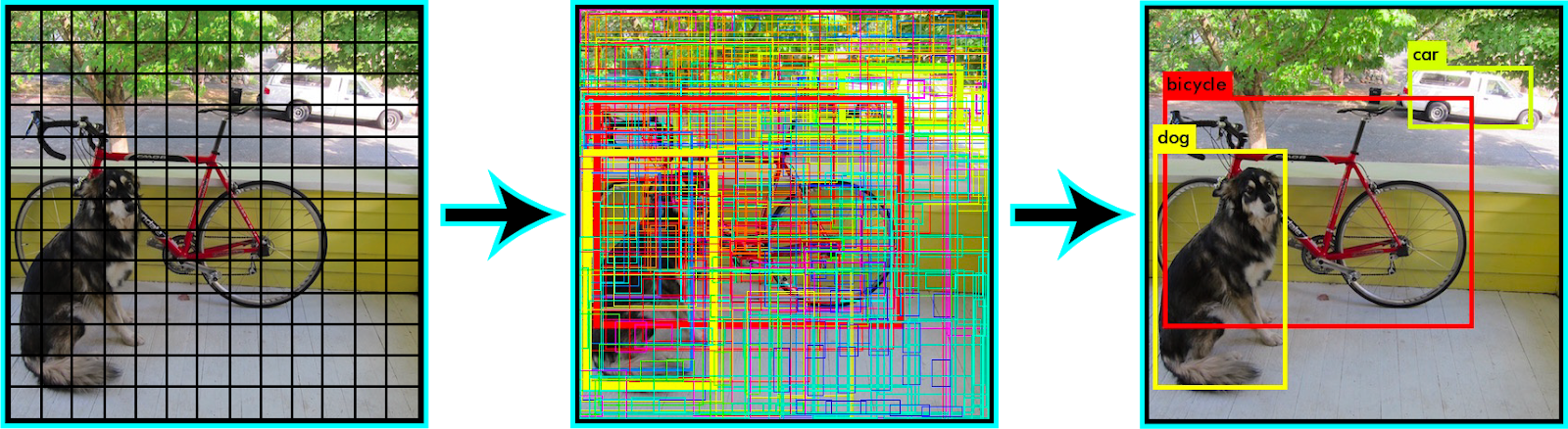
In this step, the complete (whole) frame is divided into smaller boxes or grids.
All the grids are drawn over the original image sharing the exact shape and size. The idea behind these divisions is that each grid box will detect the different objects inside it.
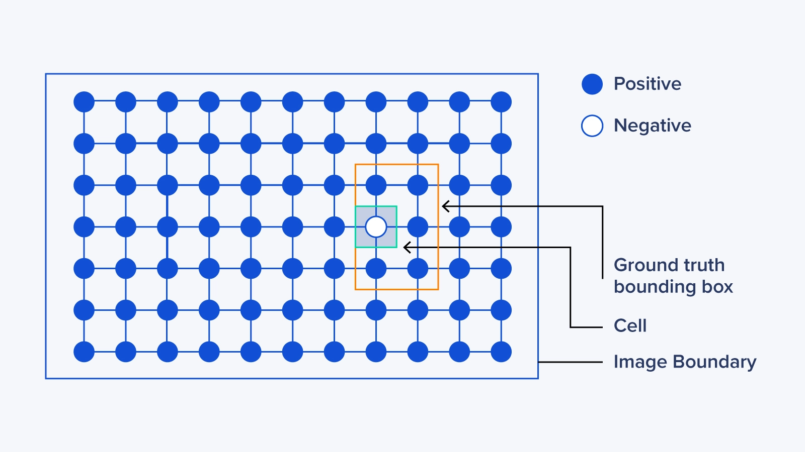
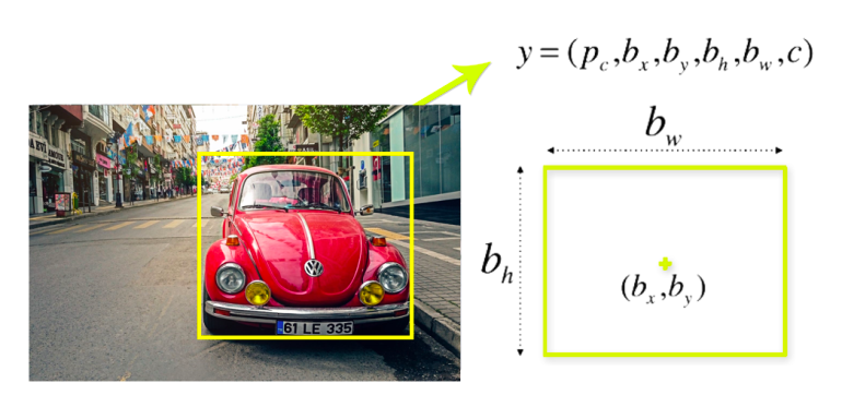
After detecting a given object in an image, a bounding box is drawn surrounding it. The bounding box has parameters such as the center point, height, width, and class (object type detected).
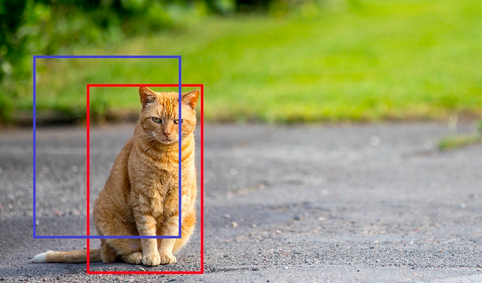
The IOU, short for intersection over union, is used to calculate our model's accuracy. This is achieved by quantifying the degree of intersection of two boxes which are the real value box (red box in image) and the box returned from our result (blue box in image).
In the tutorial portion of this article, we identified our IOU value as 40 percent, meaning that if the intersection of the two boxes is below 40 percent, then this prediction should not be taken into consideration. This is done to help us calculate the accuracy of our predictions.
Below is an image showing the complete process of the YOLO detection algorithm:
With the latest CPUs and most powerful GPUs available, accelerate your deep learning and AI project optimized to your deployment, budget, and desired performance!
Configure NowNote: You can view the original code used in this example on Kaggle.
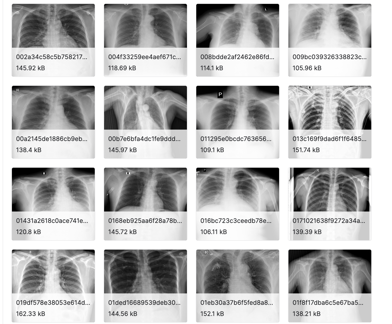
The main goal of the example in this tutorial is to use the YOLO algorithm to detect a list of chest diseases in a given image. As with any machine learning model, we will run ours using thousands of chest-scanned images. The goal is for the YOLO algorithm to successfully detect all lesions in the given image.
The VinBigData 512 image Dataset used in this tutorial can be found on Kaggle. The data set is divided into two parts, the training, and the testing data sets. The training data set contains 15,000 images, while the testing data set contains 3,000. This division of data between the training and the testing is somehow optimal as the training data set is usually 4 to 5 times the size of the testing data set.
The other part of the data set contains the label for all the images. Inside this data set each image is labeled with a class name (chest disease found), along with the class ID, width and height of the image, etc.
To start with, we will import the required libraries and packages at the very beginning of our code. First, let's explain some of the more common libraries that we just imported. NumPy is an open-source numerical Python library that allows users to create matrices and perform a number of mathematical operations on them.
import pandas as pd
import os
import numpy as np
import shutil
import ast
from sklearn import model_selection
from tqdm import tqdm
import wandb
from sklearn.model_selection import GroupKFold\
from IPython.display import Image, clear_output  # to display images
from os import listdir
from os.path import isfile
from glob import glob
import yaml
# clear_output()
To make our life easier, we will start by defining the direct paths to the labels and the images of the training and testing data sets.
TRAIN_LABELS_PATH = './vinbigdata/labels/train'
VAL_LABELS_PATH = './vinbigdata/labels/val'
TRAIN_IMAGES_PATH = './vinbigdata/images/train' #12000
VAL_IMAGES_PATH = './vinbigdata/images/val' #3000
External_DIR = '../input/vinbigdata-512-image-dataset/vinbigdata/train' # 15000
os.makedirs(TRAIN_LABELS_PATH, exist_ok = True)
os.makedirs(VAL_LABELS_PATH, exist_ok = True)
os.makedirs(TRAIN_IMAGES_PATH, exist_ok = True)
os.makedirs(VAL_IMAGES_PATH, exist_ok = True)
size = 51
Here we will import and read the textual data set. This data is stored as rows and columns in a CSV file format.
df = pd.read_csv('../input/vinbigdata-512-image-dataset/vinbigdata/train.csv')
df.head()
Note: the df.head() function prints the first 5 rows of the given data set.
As no data set is perfect, most of the time a filtering process is necessary to optimize a data set, thus optimizing our model’s performance. In this step, we would drop any row with a class id that is equal to 14.
This class id stands for a no finding in the disease class. The reason we dropped this class is that it may confuse our model. Moreover, it will slow it down because our data set will be slightly bigger.
df = df[df.class_id!=14].reset_index(drop = True)
As mentioned previously in the 'How does the YOLO algorithm work section' (particularly steps 1 and 2), the YOLO algorithm expects the dataset to be in a certain format. Here we will be going through the dataframe and applying a few transformations.
The end goal of the below code is to calculate the new x-mid, y-mid, width, and height dimensions for each data point.
df['x_min'] = df.apply(lambda row: (row.x_min)/row.width, axis = 1)*float(size)
df['y_min'] = df.apply(lambda row: (row.y_min)/row.height, axis = 1)*float(size)
df['x_max'] = df.apply(lambda row: (row.x_max)/row.width, axis =1)*float(size)
df['y_max'] = df.apply(lambda row: (row.y_max)/row.height, axis =1)*float(size)

df['x_mid'] = df.apply(lambda row: (row.x_max+row.x_min)/2, axis =1)
df['y_mid'] = df.apply(lambda row: (row.y_max+row.y_min)/2, axis =1)

df['w'] = df.apply(lambda row: (row.x_max-row.x_min), axis =1)
df['h'] = df.apply(lambda row: (row.y_max-row.y_min), axis =1)

df['x_mid'] /= float(size)
df['y_mid'] /= float(size)

df['w'] /= float(size)
df['h'] /= float(size)
In this part of the code, we will change the given data format of all rows in the dataset into the following columns; <class> <x_center> <y_center> <width> <height>.This is necessary since the YOLOv5 algorithm can only read the data in this specific format.
# <class> <x_center> <y_center> <width> <height>
def preproccess_data(df, labels_path, images_path):
    for column, row in tqdm(df.iterrows(), total=len(df)):
        attributes = row[['class_id','x_mid','y_mid','w','h']].values
        attributes = np.array(attributes)
        np.savetxt(os.path.join(labels_path, f"{row['image_id']}.txt"),
                   [attributes], fmt = ['%d', '%f', '%f', '%f', '%f'])
        shutil.copy(os.path.join('/kaggle/input/vinbigdata-512-image-dataset/vinbigdata/train', f"{row['image_id']}.png"),images_path)
We will then run the preproccess_data function two times, once with the training data set and its images, and the second with the testing data set and its images.
preproccess_data(df, TRAIN_LABELS_PATH, TRAIN_IMAGES_PATH)
preproccess_data(val_df, VAL_LABELS_PATH, VAL_IMAGES_PATH)
Using the line below, we will clone the YOLOv5 algorithm into our model.
!git clone https://github.com/ultralytics/yolov5.git
Here we will define the available 14 chest diseases in our models as classes. These are the actual diseases that can be identified in the data set’s images.
classes = [
	'Aortic enlargement',
	'Atelectasis',
	'Calcification',
	'Cardiomegaly',
	'Consolidation',
	'ILD',
	'Infiltration',
	'Lung Opacity',
	'Nodule/Mass',
	'Other lesion',
	'Pleural effusion',
	'Pleural thickening',
	'Pneumothorax',
	'Pulmonary fibrosis'
	]

data = dict(
    train =  '../vinbigdata/images/train',
    val   =  '../vinbigdata/images/val',
    nc    = 14,
    names = classes
    )

with open('./yolov5/vinbigdata.yaml', 'w') as outfile:
    yaml.dump(data, outfile, default_flow_style=False)

f = open('./yolov5/vinbigdata.yaml', 'r')
print('\nyaml:')
print(f.read())
To start, we will open the YOLOv5 directory. Then we will use pip in order to install all the libraries written inside the requirements file.
The requirements file contains all the required libraries that the code base needs to work. We will also install other libraries such as pycocotools, seaborn, and pandas.
%cd ./yolov5
!pip install -U -r requirements.txt
!pip install pycocotools>=2.0 seaborn>=0.11.0 pandas thop
clear_output()
Wandb, short for weights and biases, allows us to monitor a given neural network model.
# b39dd18eed49a73a53fccd7b684ea7ecaed75b08
wandb.login()
Now we will train the YOLOv5 on the vinbigdata set provided for 100 epochs. We’ll also pass some other flags such as --img 512 which tells the model that our image size is 512 pixels, --batch 16 will allow our model to take 16images per batch. Using the --data ./vinbigdata.yaml flag we will pass our dataset which is the vinbigdata.yaml data set.
!python train.py --img 512 --batch 16 --epochs 100 --data ./vinbigdata.yaml --cfg models/yolov5x.yaml --weights yolov5x.pt --cache --name vin

Training AI models on massive datasets can be accelerated exponentially with the right system. It's not just a high-performance computer, but a tool to propel and accelerate your research.
Configure NowFirst, we will identify the testing data set directory along with the weights directory.
test_dir = f'/kaggle/input/vinbigdata-{size}-image-dataset/vinbigdata/test'
weights_dir = './runs/train/vin3/weights/best.pt'
os.listdir('./runs/train/vin3/weights')
In this part, we will use the detect.py as our inference to check the accuracy of our predictions. We will also pass some flags such as --conf 0.15\ which is the model's confidence threshold. If the confidence rate of a detected object is under 15 percent then remove it from our output. The --iou 0.4\ flag informs our model that if the intersection over the union of two boxes is below 40 percent then it should be removed.
!python detect.py --weights $weights_dir\
--img 512\
--conf 0.15\
--iou 0.4\
--source $test_dir\
--save-txt --save-conf --exist-ok
In this article, we explained what YOLOv5 is and how the basic YOLO algorithm works. Next, we went on to briefly explain PyTorch. Then we covered a couple of reasons why you should use YOLO over other, similar detection algorithms.
Finally, we walked you through a machine-learning model that is capable of detecting chest diseases in x-ray images. In this example, we used YOLO as our main detection algorithm to find and locate chest lesions. We then classified each lesion into a given class or disease.
If you are interested in machine learning and building your own models, especially models that require the detection of multiple objects in a given image or video representation, then YOLOv5 is definitely worth a try. If you're looking to build or source an AI Training Workstation or Server, contact Exxact to configure one today!
YOLO, an acronym for 'You only look once,’ is an open-source software tool utilized for its efficient capability of detecting objects in a given image in real time. The YOLO algorithm uses convolutional neural network (CNN) models to detect objects in an image.
The algorithm requires only one forward propagation through a given neural network to detect all objects in the image. This gives the YOLO algorithm an edge in speed over others, making it one of the most well-known detection algorithms to date.
An object detection algorithm is an algorithm that is capable of detecting certain objects or shapes in a given frame. For example, simple detection algorithms may be capable of detecting and identifying shapes in an image such as circles or squares, while more advanced detection algorithms can detect more complex objects such as humans, bicycles, cars, etc.
Not only does the YOLO algorithm offer high detection speed and performance through its one-forward propagation capability, but it also detects them with great accuracy and precision.
In this tutorial, we will focus on YOLOv5, which is the fifth and latest version of the YOLO software. It was originally released on the 18th of May 2020. The YOLO open-source code can be found on GitHub. We will be using YOLO with the well-known PyTorch library.
PyTorch is a deep learning open-source package that is based on the well-known Torch library. It's also a Python-based library that is more commonly used for natural language processing and computer vision.
In this step, the complete (whole) frame is divided into smaller boxes or grids.
All the grids are drawn over the original image sharing the exact shape and size. The idea behind these divisions is that each grid box will detect the different objects inside it.
After detecting a given object in an image, a bounding box is drawn surrounding it. The bounding box has parameters such as the center point, height, width, and class (object type detected).
The IOU, short for intersection over union, is used to calculate our model's accuracy. This is achieved by quantifying the degree of intersection of two boxes which are the real value box (red box in image) and the box returned from our result (blue box in image).
In the tutorial portion of this article, we identified our IOU value as 40 percent, meaning that if the intersection of the two boxes is below 40 percent, then this prediction should not be taken into consideration. This is done to help us calculate the accuracy of our predictions.
Below is an image showing the complete process of the YOLO detection algorithm:
With the latest CPUs and most powerful GPUs available, accelerate your deep learning and AI project optimized to your deployment, budget, and desired performance!
Configure NowNote: You can view the original code used in this example on Kaggle.
The main goal of the example in this tutorial is to use the YOLO algorithm to detect a list of chest diseases in a given image. As with any machine learning model, we will run ours using thousands of chest-scanned images. The goal is for the YOLO algorithm to successfully detect all lesions in the given image.
The VinBigData 512 image Dataset used in this tutorial can be found on Kaggle. The data set is divided into two parts, the training, and the testing data sets. The training data set contains 15,000 images, while the testing data set contains 3,000. This division of data between the training and the testing is somehow optimal as the training data set is usually 4 to 5 times the size of the testing data set.
The other part of the data set contains the label for all the images. Inside this data set each image is labeled with a class name (chest disease found), along with the class ID, width and height of the image, etc.
To start with, we will import the required libraries and packages at the very beginning of our code. First, let's explain some of the more common libraries that we just imported. NumPy is an open-source numerical Python library that allows users to create matrices and perform a number of mathematical operations on them.
import pandas as pd
import os
import numpy as np
import shutil
import ast
from sklearn import model_selection
from tqdm import tqdm
import wandb
from sklearn.model_selection import GroupKFold\
from IPython.display import Image, clear_output  # to display images
from os import listdir
from os.path import isfile
from glob import glob
import yaml
# clear_output()
To make our life easier, we will start by defining the direct paths to the labels and the images of the training and testing data sets.
TRAIN_LABELS_PATH = './vinbigdata/labels/train'
VAL_LABELS_PATH = './vinbigdata/labels/val'
TRAIN_IMAGES_PATH = './vinbigdata/images/train' #12000
VAL_IMAGES_PATH = './vinbigdata/images/val' #3000
External_DIR = '../input/vinbigdata-512-image-dataset/vinbigdata/train' # 15000
os.makedirs(TRAIN_LABELS_PATH, exist_ok = True)
os.makedirs(VAL_LABELS_PATH, exist_ok = True)
os.makedirs(TRAIN_IMAGES_PATH, exist_ok = True)
os.makedirs(VAL_IMAGES_PATH, exist_ok = True)
size = 51
Here we will import and read the textual data set. This data is stored as rows and columns in a CSV file format.
df = pd.read_csv('../input/vinbigdata-512-image-dataset/vinbigdata/train.csv')
df.head()
Note: the df.head() function prints the first 5 rows of the given data set.
As no data set is perfect, most of the time a filtering process is necessary to optimize a data set, thus optimizing our model’s performance. In this step, we would drop any row with a class id that is equal to 14.
This class id stands for a no finding in the disease class. The reason we dropped this class is that it may confuse our model. Moreover, it will slow it down because our data set will be slightly bigger.
df = df[df.class_id!=14].reset_index(drop = True)
As mentioned previously in the 'How does the YOLO algorithm work section' (particularly steps 1 and 2), the YOLO algorithm expects the dataset to be in a certain format. Here we will be going through the dataframe and applying a few transformations.
The end goal of the below code is to calculate the new x-mid, y-mid, width, and height dimensions for each data point.
df['x_min'] = df.apply(lambda row: (row.x_min)/row.width, axis = 1)*float(size)
df['y_min'] = df.apply(lambda row: (row.y_min)/row.height, axis = 1)*float(size)
df['x_max'] = df.apply(lambda row: (row.x_max)/row.width, axis =1)*float(size)
df['y_max'] = df.apply(lambda row: (row.y_max)/row.height, axis =1)*float(size)

df['x_mid'] = df.apply(lambda row: (row.x_max+row.x_min)/2, axis =1)
df['y_mid'] = df.apply(lambda row: (row.y_max+row.y_min)/2, axis =1)

df['w'] = df.apply(lambda row: (row.x_max-row.x_min), axis =1)
df['h'] = df.apply(lambda row: (row.y_max-row.y_min), axis =1)

df['x_mid'] /= float(size)
df['y_mid'] /= float(size)

df['w'] /= float(size)
df['h'] /= float(size)
In this part of the code, we will change the given data format of all rows in the dataset into the following columns; <class> <x_center> <y_center> <width> <height>.This is necessary since the YOLOv5 algorithm can only read the data in this specific format.
# <class> <x_center> <y_center> <width> <height>
def preproccess_data(df, labels_path, images_path):
    for column, row in tqdm(df.iterrows(), total=len(df)):
        attributes = row[['class_id','x_mid','y_mid','w','h']].values
        attributes = np.array(attributes)
        np.savetxt(os.path.join(labels_path, f"{row['image_id']}.txt"),
                   [attributes], fmt = ['%d', '%f', '%f', '%f', '%f'])
        shutil.copy(os.path.join('/kaggle/input/vinbigdata-512-image-dataset/vinbigdata/train', f"{row['image_id']}.png"),images_path)
We will then run the preproccess_data function two times, once with the training data set and its images, and the second with the testing data set and its images.
preproccess_data(df, TRAIN_LABELS_PATH, TRAIN_IMAGES_PATH)
preproccess_data(val_df, VAL_LABELS_PATH, VAL_IMAGES_PATH)
Using the line below, we will clone the YOLOv5 algorithm into our model.
!git clone https://github.com/ultralytics/yolov5.git
Here we will define the available 14 chest diseases in our models as classes. These are the actual diseases that can be identified in the data set’s images.
classes = [
	'Aortic enlargement',
	'Atelectasis',
	'Calcification',
	'Cardiomegaly',
	'Consolidation',
	'ILD',
	'Infiltration',
	'Lung Opacity',
	'Nodule/Mass',
	'Other lesion',
	'Pleural effusion',
	'Pleural thickening',
	'Pneumothorax',
	'Pulmonary fibrosis'
	]

data = dict(
    train =  '../vinbigdata/images/train',
    val   =  '../vinbigdata/images/val',
    nc    = 14,
    names = classes
    )

with open('./yolov5/vinbigdata.yaml', 'w') as outfile:
    yaml.dump(data, outfile, default_flow_style=False)

f = open('./yolov5/vinbigdata.yaml', 'r')
print('\nyaml:')
print(f.read())
To start, we will open the YOLOv5 directory. Then we will use pip in order to install all the libraries written inside the requirements file.
The requirements file contains all the required libraries that the code base needs to work. We will also install other libraries such as pycocotools, seaborn, and pandas.
%cd ./yolov5
!pip install -U -r requirements.txt
!pip install pycocotools>=2.0 seaborn>=0.11.0 pandas thop
clear_output()
Wandb, short for weights and biases, allows us to monitor a given neural network model.
# b39dd18eed49a73a53fccd7b684ea7ecaed75b08
wandb.login()
Now we will train the YOLOv5 on the vinbigdata set provided for 100 epochs. We’ll also pass some other flags such as --img 512 which tells the model that our image size is 512 pixels, --batch 16 will allow our model to take 16images per batch. Using the --data ./vinbigdata.yaml flag we will pass our dataset which is the vinbigdata.yaml data set.
!python train.py --img 512 --batch 16 --epochs 100 --data ./vinbigdata.yaml --cfg models/yolov5x.yaml --weights yolov5x.pt --cache --name vin
Training AI models on massive datasets can be accelerated exponentially with the right system. It's not just a high-performance computer, but a tool to propel and accelerate your research.
Configure NowFirst, we will identify the testing data set directory along with the weights directory.
test_dir = f'/kaggle/input/vinbigdata-{size}-image-dataset/vinbigdata/test'
weights_dir = './runs/train/vin3/weights/best.pt'
os.listdir('./runs/train/vin3/weights')
In this part, we will use the detect.py as our inference to check the accuracy of our predictions. We will also pass some flags such as --conf 0.15\ which is the model's confidence threshold. If the confidence rate of a detected object is under 15 percent then remove it from our output. The --iou 0.4\ flag informs our model that if the intersection over the union of two boxes is below 40 percent then it should be removed.
!python detect.py --weights $weights_dir\
--img 512\
--conf 0.15\
--iou 0.4\
--source $test_dir\
--save-txt --save-conf --exist-ok
In this article, we explained what YOLOv5 is and how the basic YOLO algorithm works. Next, we went on to briefly explain PyTorch. Then we covered a couple of reasons why you should use YOLO over other, similar detection algorithms.
Finally, we walked you through a machine-learning model that is capable of detecting chest diseases in x-ray images. In this example, we used YOLO as our main detection algorithm to find and locate chest lesions. We then classified each lesion into a given class or disease.
If you are interested in machine learning and building your own models, especially models that require the detection of multiple objects in a given image or video representation, then YOLOv5 is definitely worth a try. If you're looking to build or source an AI Training Workstation or Server, contact Exxact to configure one today!