Deep Learning
Building a Computer Vision Model Using TensorFlow
August 22, 2022
17 min read


Computer vision (CV) is a major task for modern Artificial Intelligence (AI) and Machine Learning (ML) systems. It is accelerating almost every domain in the industry enabling organizations to revolutionize the way machines and business systems work.
Academically, it is a well-established area of computer science and many decades' worth of research work have gone into this field to make it rich. The use of deep neural networks has recently revolutionized the field and given it new life.
There is a diverse array of application areas for computer vision such as:
Is your current system not cutting it? Exxact offers custom-tailored workstations and servers to speed up AI and deep learning development at compelling pricing and lighting quick turnaround.
There are, of course, plenty of challenges associated with CV systems. For example, autonomous driving doesn’t just use object detection but also object classification, segmentation, motion detection, etc.
On top of it, these systems are expected to process CV information in a fraction of a second and produce a high-probability decision. The higher-level supervisory control system has to make the decision, responsible for the ultimate driving task.
Furthermore, multiple CV systems/algorithms are often at play in any respectable autonomous driving system. The demand for parallel processing is high in those situations and this leads to high stress on the underlying computing machinery.
If multiple neural networks are used at the same time, they may be sharing the common system storage and compete with each other for a common pool of resources.
In the case of medical imaging, the performance of the computer vision system is judged by highly experienced radiologists and clinical professionals who understand the pathology behind an image. Moreover, in most cases, the task involves identifying rare diseases with very low prevalence rates.
This makes the training-data sparse and rarefied i.e. not enough training images can be found. Consequently, the Deep Learning (DL) architecture has to compensate for this by adding clever processing and architectural complexity.
TensorFlow is a widely used and highly regarded open-source Python package from Google that makes building computer vision deep learning models straightforward and easy. From its official website:
“It has a comprehensive, flexible ecosystem of tools, libraries, and community resources that lets researchers push the state-of-the-art in ML and developers easily build and deploy ML-powered applications”.
With the release of TensorFlow 2.0 and Keras library integration as the high-level API, it is easy to stack layers of neurons and build and train deep learning architectures of sufficient complexity.
|
|
|
Easy Model Building Build and train ML, models easily using intuitive high level APIs like Keras for immediate model iteration and easy debugging | Robust ML Production Anywhere Easily train and deploy models in the cloud, on-prem, on on-device, no matter what programing language you use. | Powerful for Research Simple and flexible architecture to take new ideas from concept to code. Publish state-of-the-art models with confidence |
Now, of course, TensorFlow can be used to build deep learning models for all kinds of applications including,
However, in this article, we focus on code and hands-on examples of building a simple object classification task with Convolutional Neural Network (CNN) using TensorFlow.
This covers all the essential components of TensorFlow such as layers, optimizers, error functions, training options, hyperparameter tuning, etc.
Deep learning tasks and model training benefit extensively from specialized hardware like Gaming Processing Units (GPU).
General-purpose CPUs struggle when operating on a large amount of data e.g., performing linear algebra operations on matrices with tens or hundreds of thousand floating-point numbers.
Under the hood, deep neural networks are mostly composed of operations like matrix multiplications and vector additions.GPUs were developed (primarily catering to the video gaming industry) to handle a massive degree of parallel computations using thousands of tiny computing cores.
They also feature large memory bandwidth to deal with the rapid dataflow (processing unit to cache to the slower main memory and back), needed for these computations when the neural network is training through hundreds of epochs. This makes them the ideal commodity hardware to deal with the computation load of computer vision tasks.
There are various avenues to use a GPU for deep learning tasks. Purchasing a bare metal server, or workstation can be beneficial for those looking for peak customizability. Renting GPU computing resources on Cloud from AWS or GCP is great for those running short sessions with limited data. Or use free (but limited) resources like Google Colaboratory. The larger the dataset, the better the model but in this example, we use the last option Google Colab.
We first test whether a GPU is present for training,
import tensorflow as tf
device_name = tf.test.gpu_device_name()

if device_name != '/device:GPU:0':
  raise SystemError('GPU device not found')

print('Found GPU at: {}'.format(device_name))
We directly download the dataset into the local environment (of Google Colab) with the following code. If you are working on your local machine (and saved the file already), then modify the code accordingly.
!wget --no-check-certificate \ https://storage.googleapis.com/laurencemoroney-blog.appspot.com/horse-or-human.zip \
-O /tmp/horse-or-human.zip
The following python code will use the OS library to use Operating System libraries, giving you access to the file system, and the zipfile library allowing you to unzip the data.
import os
import zipfile

local_zip = '/tmp/horse-or-human.zip'
zip_ref = zipfile.ZipFile(local_zip, 'r')

zip_ref.extractall('/tmp/horse-or-human')
zip_ref.close()
The contents of the .zip are extracted to the base directory /tmp/horse-or-human, which in turn each contains horses and humans subdirectories. In short, the training set is the data that is used to tell the neural network model that 'this is what a horse looks like', ' this is what a human looks like' etc.
Note that we do not explicitly label the images as horses or humans. Later we will see something called an ImageGenerator being used -- and this is coded to read images from subdirectories, and automatically label them from the name of that subdirectory. So, for example, we will have a 'training' directory containing a 'horses' directory and a 'humans' one. ImageGenerator will label the images appropriately for you, reducing the coding step.
Let's define each of these directories.
# Directory with our training horse pictures
train_horse_dir = os.path.join('/tmp/horse-or-human/horses')

# Directory with our training human pictures
train_human_dir = os.path.join('/tmp/horse-or-human/humans')
The following code will let us see what the filenames look like in the horses and humans training directories.
train_horse_names = os.listdir(train_horse_dir)
print(train_horse_names[:10])

train_human_names = os.listdir(train_human_dir)
print(train_human_names[:10])
We can find out the total number of horse and human images in the directories.
print('total training horse images:', len(os.listdir(train_horse_dir)))
print('total training human images:', len(os.listdir(train_human_dir)))
Now let's take a look at a few pictures to get a better sense of what they look like. We, first configure the matplot parameters,
<a data-re-name="format" data-dropdown="true" href="https://app.contentstack.com/#" alt="Format" rel="format" role="button" aria-label="Format" tabindex="-1" data-re-icon="true"></a>
import matplotlib.pyplot as plt
import matplotlib.image as mpimg

# Parameters for our graph; we'll output images in a 4x4 configuration
nrows = 4
ncols = 4

# Index for iterating over images
pic_index = 0
Now, display a batch of 8 horse and 8 human pictures. We can rerun the following code in a Jupyter notebook cell to see a fresh batch each time.
# Set up matplotlib fig, and size it to fit 4x4 pics
fig = plt.gcf()

fig.set_size_inches(ncols * 4, nrows * 4)

pic_index += 8
next_horse_pix = [os.path.join(train_horse_dir, fname)
                for fname in train_horse_names[pic_index-8:pic_index]]

next_human_pix = [os.path.join(train_human_dir, fname)
                for fname in train_human_names[pic_index-8:pic_index]]

for i, img_path in enumerate(next_horse_pix+next_human_pix):
  # Set up subplot; subplot indices start at 1
  sp = plt.subplot(nrows, ncols, i + 1)
  sp.axis('Off') # Don't show axes (or gridlines)

  img = mpimg.imread(img_path)
  plt.imshow(img)

plt.show()
First, import the TensorFlow library,
import tensorflow as tf
We then add convolutional layers and flatten the final result to feed into the densely connected layers. Finally, we add the densely connected layers.
Note: We are facing a two-class classification problem, i.e. a binary classification problem, we will end our network with a sigmoid activation, so that the output of our network will be a single scalar between 0 and 1, encoding the probability that the current image is class 1 (as opposed to class 0).
model = tf.keras.models.Sequential([
# Note the input shape is the desired size of the image 300x300 with 3 bytes color

# This is the first convolution
tf.keras.layers.Conv2D(16, (3,3), activation='relu', input_shape=(300, 300, 3)),
tf.keras.layers.MaxPooling2D(2, 2),

# The second convolution
tf.keras.layers.Conv2D(32, (3,3), activation='relu'),
tf.keras.layers.MaxPooling2D(2,2),

# The third convolution
tf.keras.layers.Conv2D(64, (3,3), activation='relu'),
tf.keras.layers.MaxPooling2D(2,2),

# The fourth convolution
tf.keras.layers.Conv2D(64, (3,3), activation='relu'),
tf.keras.layers.MaxPooling2D(2,2),

# The fifth convolution
tf.keras.layers.Conv2D(64, (3,3), activation='relu'),
tf.keras.layers.MaxPooling2D(2,2),

# Flatten the results to feed into a DNN
tf.keras.layers.Flatten(),

# 512 neuron hidden layer
tf.keras.layers.Dense(512, activation='relu'),

# Only 1 output neuron. It will contain a value from 0-1 where 0 for 1 class ('horses') and 1 for the other ('humans')
tf.keras.layers.Dense(1, activation='sigmoid')
])
Note the use of tf.keras API for building the model. The model.summary() method call prints a summary of the neural network.
The "output shape" column shows how the size of your feature map evolves in each successive layer. The convolution layers reduce the size of the feature maps by a bit due to padding, and each pooling layer halves the dimensions.
Next, we'll configure the specifications for model training. We will train our model with the binary_crossentropy loss because it's a binary classification problem and our final activation is a sigmoid. (For a refresher on loss metrics, see the Machine Learning Crash Course.) We will use the rmsprop optimizer with a learning rate of 0.001.
During training, we will want to monitor classification accuracy. NOTE: In this case, using the RMSprop optimization algorithm is preferable to stochastic gradient descent (SGD), because rmsprop automates learning-rate tuning for us.
Other optimizers, such as Adam and Adagrad, also automatically adapt the learning rate during training and would work equally well here.
from tensorflow.keras.optimizers import RMSprop

model.compile(loss='binary_crossentropy',
              optimizer=RMSprop(lr=0.001),
              metrics=['acc'])
Let's set up data generators that will read pictures in our source folders, convert them to float32 tensors, and feed them (with their labels) to our network. We'll have one generator for the training images and one for the validation images. Our generators will yield batches of images of size 300x300 and their labels (binary).
As you may already know, data that goes into neural networks should usually be normalized in some way to make it more amenable to processing by the network. (It is uncommon to feed raw pixels into a convnet.)
In our case, we will preprocess our images by normalizing the pixel values to be in the [0, 1] range (originally all values are in the [0, 255] range).
In Keras, this can be done using the rescale parameter:
keras.preprocessing.image.ImageDataGenerator
This ImageDataGenerator class allows you to instantiate generators of augmented image batches (and their labels) via .flow(data, labels) or .flow_from_directory(directory).
These generators can then be used with the Keras model methods that accept data generators as inputs: fit_generator, evaluate_generator, and predict_generator.
from tensorflow.keras.preprocessing.image import ImageDataGenerator

# All images will be rescaled by 1./255
train_datagen = ImageDataGenerator(rescale=1/255)

# Flow training images in batches of 128 using train_datagen generator
train_generator = train_datagen.flow_from_directory(
        '/tmp/horse-or-human/', # This is the source directory for training images
        target_size=(300, 300), # All images will be resized to 300x300
        batch_size=128,
        # Since we use binary_crossentropy loss, we need binary labels
        class_mode='binary')
Let's train for 15 epochs -- this may take a few minutes to run on a typical Google Colab hardware. The Loss and Accuracy are a great indication of progress of training. It's making a guess as to the classification of the training data, and then measuring it against the known label, calculating the result. Accuracy is the fraction/percentage of correct predictions.
history = model.fit_generator(
      train_generator,
      steps_per_epoch=8,
      epochs=15,
      verbose=2)
The following code will help us plot the accuracy graph i.e., how the accuracy has improved with repeated training (passing the images through the network back and forth) epochs.
plt.plot(history.history['acc'],c='k',lw=2)
plt.grid(True)
plt.title("Training accuracy with epochs\n",fontsize=18)
plt.xlabel("Training epochs",fontsize=15)
plt.ylabel("Training accuracy",fontsize=15)
plt.show()
Let's now take a look at actually running a prediction using the model. This code will allow you to choose 1 or more files from your file system, it will then upload them, and run them through the model, indicating whether the object is a horse or a human. For this purpose, we use files.upload() method from the google.colab class.
NOTE: Please download some images of horses and humans from the internet and keep them on your local hard drive as you will need to upload them for testing the model. You can upload multiple images at a time.
import numpy as np
from google.colab import files
from keras.preprocessing import image

uploaded = files.upload()

for fn in uploaded.keys():
  # predicting images
  path = '/content/' + fn
  img = image.load_img(path, target_size=(300, 300))
  plt.imshow(img)
  plt.show()
  x = image.img_to_array(img)
  x = np.expand_dims(x, axis=0)

images = np.vstack([x])
  classes = model.predict(images, batch_size=10)
  if classes[0]>0.5:
    print(fn + " shows a human image")
  else:
    print(fn + " shows a horse image")
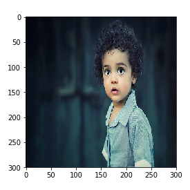
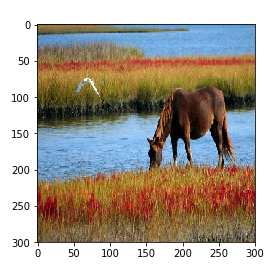
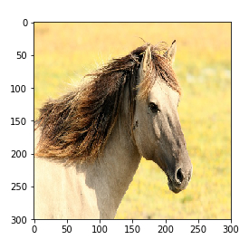
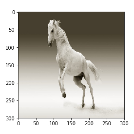
Here are some example test images. If trained properly, the network will predict ‘human’ class for the first one and ‘horse’ class for the other three.
|
|
|
|
The model got some right but some wrong. The model has a high chance of making a mistake in the last image. You are encouraged to test with your images and check the performance of the model.
In this article, we covered building a computer vision model with convolutional neural net architecture using the TensorFlow and Keras framework for an object classification task.
Hands-on code was provided and all the important components of TensorFlow - layers, model compile, optimizers, loss functions, and even Image generator class - were covered in this one example. Take this as a starting point and explore many more CV tasks using TensorFlow such as object detection, semantic segmentation, etc.
Have any questions?
Contact Exxact to learn more!
Computer vision (CV) is a major task for modern Artificial Intelligence (AI) and Machine Learning (ML) systems. It is accelerating almost every domain in the industry enabling organizations to revolutionize the way machines and business systems work.
Academically, it is a well-established area of computer science and many decades' worth of research work have gone into this field to make it rich. The use of deep neural networks has recently revolutionized the field and given it new life.
There is a diverse array of application areas for computer vision such as:
Is your current system not cutting it? Exxact offers custom-tailored workstations and servers to speed up AI and deep learning development at compelling pricing and lighting quick turnaround.
There are, of course, plenty of challenges associated with CV systems. For example, autonomous driving doesn’t just use object detection but also object classification, segmentation, motion detection, etc.
On top of it, these systems are expected to process CV information in a fraction of a second and produce a high-probability decision. The higher-level supervisory control system has to make the decision, responsible for the ultimate driving task.
Furthermore, multiple CV systems/algorithms are often at play in any respectable autonomous driving system. The demand for parallel processing is high in those situations and this leads to high stress on the underlying computing machinery.
If multiple neural networks are used at the same time, they may be sharing the common system storage and compete with each other for a common pool of resources.
In the case of medical imaging, the performance of the computer vision system is judged by highly experienced radiologists and clinical professionals who understand the pathology behind an image. Moreover, in most cases, the task involves identifying rare diseases with very low prevalence rates.
This makes the training-data sparse and rarefied i.e. not enough training images can be found. Consequently, the Deep Learning (DL) architecture has to compensate for this by adding clever processing and architectural complexity.
TensorFlow is a widely used and highly regarded open-source Python package from Google that makes building computer vision deep learning models straightforward and easy. From its official website:
“It has a comprehensive, flexible ecosystem of tools, libraries, and community resources that lets researchers push the state-of-the-art in ML and developers easily build and deploy ML-powered applications”.
With the release of TensorFlow 2.0 and Keras library integration as the high-level API, it is easy to stack layers of neurons and build and train deep learning architectures of sufficient complexity.
|
|
|
Easy Model Building Build and train ML, models easily using intuitive high level APIs like Keras for immediate model iteration and easy debugging | Robust ML Production Anywhere Easily train and deploy models in the cloud, on-prem, on on-device, no matter what programing language you use. | Powerful for Research Simple and flexible architecture to take new ideas from concept to code. Publish state-of-the-art models with confidence |
Now, of course, TensorFlow can be used to build deep learning models for all kinds of applications including,
However, in this article, we focus on code and hands-on examples of building a simple object classification task with Convolutional Neural Network (CNN) using TensorFlow.
This covers all the essential components of TensorFlow such as layers, optimizers, error functions, training options, hyperparameter tuning, etc.
Deep learning tasks and model training benefit extensively from specialized hardware like Gaming Processing Units (GPU).
General-purpose CPUs struggle when operating on a large amount of data e.g., performing linear algebra operations on matrices with tens or hundreds of thousand floating-point numbers.
Under the hood, deep neural networks are mostly composed of operations like matrix multiplications and vector additions.GPUs were developed (primarily catering to the video gaming industry) to handle a massive degree of parallel computations using thousands of tiny computing cores.
They also feature large memory bandwidth to deal with the rapid dataflow (processing unit to cache to the slower main memory and back), needed for these computations when the neural network is training through hundreds of epochs. This makes them the ideal commodity hardware to deal with the computation load of computer vision tasks.
There are various avenues to use a GPU for deep learning tasks. Purchasing a bare metal server, or workstation can be beneficial for those looking for peak customizability. Renting GPU computing resources on Cloud from AWS or GCP is great for those running short sessions with limited data. Or use free (but limited) resources like Google Colaboratory. The larger the dataset, the better the model but in this example, we use the last option Google Colab.
We first test whether a GPU is present for training,
import tensorflow as tf
device_name = tf.test.gpu_device_name()

if device_name != '/device:GPU:0':
  raise SystemError('GPU device not found')

print('Found GPU at: {}'.format(device_name))
We directly download the dataset into the local environment (of Google Colab) with the following code. If you are working on your local machine (and saved the file already), then modify the code accordingly.
!wget --no-check-certificate \ https://storage.googleapis.com/laurencemoroney-blog.appspot.com/horse-or-human.zip \
-O /tmp/horse-or-human.zip
The following python code will use the OS library to use Operating System libraries, giving you access to the file system, and the zipfile library allowing you to unzip the data.
import os
import zipfile

local_zip = '/tmp/horse-or-human.zip'
zip_ref = zipfile.ZipFile(local_zip, 'r')

zip_ref.extractall('/tmp/horse-or-human')
zip_ref.close()
The contents of the .zip are extracted to the base directory /tmp/horse-or-human, which in turn each contains horses and humans subdirectories. In short, the training set is the data that is used to tell the neural network model that 'this is what a horse looks like', ' this is what a human looks like' etc.
Note that we do not explicitly label the images as horses or humans. Later we will see something called an ImageGenerator being used -- and this is coded to read images from subdirectories, and automatically label them from the name of that subdirectory. So, for example, we will have a 'training' directory containing a 'horses' directory and a 'humans' one. ImageGenerator will label the images appropriately for you, reducing the coding step.
Let's define each of these directories.
# Directory with our training horse pictures
train_horse_dir = os.path.join('/tmp/horse-or-human/horses')

# Directory with our training human pictures
train_human_dir = os.path.join('/tmp/horse-or-human/humans')
The following code will let us see what the filenames look like in the horses and humans training directories.
train_horse_names = os.listdir(train_horse_dir)
print(train_horse_names[:10])

train_human_names = os.listdir(train_human_dir)
print(train_human_names[:10])
We can find out the total number of horse and human images in the directories.
print('total training horse images:', len(os.listdir(train_horse_dir)))
print('total training human images:', len(os.listdir(train_human_dir)))
Now let's take a look at a few pictures to get a better sense of what they look like. We, first configure the matplot parameters,
<a data-re-name="format" data-dropdown="true" href="https://app.contentstack.com/#" alt="Format" rel="format" role="button" aria-label="Format" tabindex="-1" data-re-icon="true"></a>
import matplotlib.pyplot as plt
import matplotlib.image as mpimg

# Parameters for our graph; we'll output images in a 4x4 configuration
nrows = 4
ncols = 4

# Index for iterating over images
pic_index = 0
Now, display a batch of 8 horse and 8 human pictures. We can rerun the following code in a Jupyter notebook cell to see a fresh batch each time.
# Set up matplotlib fig, and size it to fit 4x4 pics
fig = plt.gcf()

fig.set_size_inches(ncols * 4, nrows * 4)

pic_index += 8
next_horse_pix = [os.path.join(train_horse_dir, fname)
                for fname in train_horse_names[pic_index-8:pic_index]]

next_human_pix = [os.path.join(train_human_dir, fname)
                for fname in train_human_names[pic_index-8:pic_index]]

for i, img_path in enumerate(next_horse_pix+next_human_pix):
  # Set up subplot; subplot indices start at 1
  sp = plt.subplot(nrows, ncols, i + 1)
  sp.axis('Off') # Don't show axes (or gridlines)

  img = mpimg.imread(img_path)
  plt.imshow(img)

plt.show()
First, import the TensorFlow library,
import tensorflow as tf
We then add convolutional layers and flatten the final result to feed into the densely connected layers. Finally, we add the densely connected layers.
Note: We are facing a two-class classification problem, i.e. a binary classification problem, we will end our network with a sigmoid activation, so that the output of our network will be a single scalar between 0 and 1, encoding the probability that the current image is class 1 (as opposed to class 0).
model = tf.keras.models.Sequential([
# Note the input shape is the desired size of the image 300x300 with 3 bytes color

# This is the first convolution
tf.keras.layers.Conv2D(16, (3,3), activation='relu', input_shape=(300, 300, 3)),
tf.keras.layers.MaxPooling2D(2, 2),

# The second convolution
tf.keras.layers.Conv2D(32, (3,3), activation='relu'),
tf.keras.layers.MaxPooling2D(2,2),

# The third convolution
tf.keras.layers.Conv2D(64, (3,3), activation='relu'),
tf.keras.layers.MaxPooling2D(2,2),

# The fourth convolution
tf.keras.layers.Conv2D(64, (3,3), activation='relu'),
tf.keras.layers.MaxPooling2D(2,2),

# The fifth convolution
tf.keras.layers.Conv2D(64, (3,3), activation='relu'),
tf.keras.layers.MaxPooling2D(2,2),

# Flatten the results to feed into a DNN
tf.keras.layers.Flatten(),

# 512 neuron hidden layer
tf.keras.layers.Dense(512, activation='relu'),

# Only 1 output neuron. It will contain a value from 0-1 where 0 for 1 class ('horses') and 1 for the other ('humans')
tf.keras.layers.Dense(1, activation='sigmoid')
])
Note the use of tf.keras API for building the model. The model.summary() method call prints a summary of the neural network.
The "output shape" column shows how the size of your feature map evolves in each successive layer. The convolution layers reduce the size of the feature maps by a bit due to padding, and each pooling layer halves the dimensions.
Next, we'll configure the specifications for model training. We will train our model with the binary_crossentropy loss because it's a binary classification problem and our final activation is a sigmoid. (For a refresher on loss metrics, see the Machine Learning Crash Course.) We will use the rmsprop optimizer with a learning rate of 0.001.
During training, we will want to monitor classification accuracy. NOTE: In this case, using the RMSprop optimization algorithm is preferable to stochastic gradient descent (SGD), because rmsprop automates learning-rate tuning for us.
Other optimizers, such as Adam and Adagrad, also automatically adapt the learning rate during training and would work equally well here.
from tensorflow.keras.optimizers import RMSprop

model.compile(loss='binary_crossentropy',
              optimizer=RMSprop(lr=0.001),
              metrics=['acc'])
Let's set up data generators that will read pictures in our source folders, convert them to float32 tensors, and feed them (with their labels) to our network. We'll have one generator for the training images and one for the validation images. Our generators will yield batches of images of size 300x300 and their labels (binary).
As you may already know, data that goes into neural networks should usually be normalized in some way to make it more amenable to processing by the network. (It is uncommon to feed raw pixels into a convnet.)
In our case, we will preprocess our images by normalizing the pixel values to be in the [0, 1] range (originally all values are in the [0, 255] range).
In Keras, this can be done using the rescale parameter:
keras.preprocessing.image.ImageDataGenerator
This ImageDataGenerator class allows you to instantiate generators of augmented image batches (and their labels) via .flow(data, labels) or .flow_from_directory(directory).
These generators can then be used with the Keras model methods that accept data generators as inputs: fit_generator, evaluate_generator, and predict_generator.
from tensorflow.keras.preprocessing.image import ImageDataGenerator

# All images will be rescaled by 1./255
train_datagen = ImageDataGenerator(rescale=1/255)

# Flow training images in batches of 128 using train_datagen generator
train_generator = train_datagen.flow_from_directory(
        '/tmp/horse-or-human/', # This is the source directory for training images
        target_size=(300, 300), # All images will be resized to 300x300
        batch_size=128,
        # Since we use binary_crossentropy loss, we need binary labels
        class_mode='binary')
Let's train for 15 epochs -- this may take a few minutes to run on a typical Google Colab hardware. The Loss and Accuracy are a great indication of progress of training. It's making a guess as to the classification of the training data, and then measuring it against the known label, calculating the result. Accuracy is the fraction/percentage of correct predictions.
history = model.fit_generator(
      train_generator,
      steps_per_epoch=8,
      epochs=15,
      verbose=2)
The following code will help us plot the accuracy graph i.e., how the accuracy has improved with repeated training (passing the images through the network back and forth) epochs.
plt.plot(history.history['acc'],c='k',lw=2)
plt.grid(True)
plt.title("Training accuracy with epochs\n",fontsize=18)
plt.xlabel("Training epochs",fontsize=15)
plt.ylabel("Training accuracy",fontsize=15)
plt.show()
Let's now take a look at actually running a prediction using the model. This code will allow you to choose 1 or more files from your file system, it will then upload them, and run them through the model, indicating whether the object is a horse or a human. For this purpose, we use files.upload() method from the google.colab class.
NOTE: Please download some images of horses and humans from the internet and keep them on your local hard drive as you will need to upload them for testing the model. You can upload multiple images at a time.
import numpy as np
from google.colab import files
from keras.preprocessing import image

uploaded = files.upload()

for fn in uploaded.keys():
  # predicting images
  path = '/content/' + fn
  img = image.load_img(path, target_size=(300, 300))
  plt.imshow(img)
  plt.show()
  x = image.img_to_array(img)
  x = np.expand_dims(x, axis=0)

images = np.vstack([x])
  classes = model.predict(images, batch_size=10)
  if classes[0]>0.5:
    print(fn + " shows a human image")
  else:
    print(fn + " shows a horse image")
Here are some example test images. If trained properly, the network will predict ‘human’ class for the first one and ‘horse’ class for the other three.
|
|
|
|
The model got some right but some wrong. The model has a high chance of making a mistake in the last image. You are encouraged to test with your images and check the performance of the model.
In this article, we covered building a computer vision model with convolutional neural net architecture using the TensorFlow and Keras framework for an object classification task.
Hands-on code was provided and all the important components of TensorFlow - layers, model compile, optimizers, loss functions, and even Image generator class - were covered in this one example. Take this as a starting point and explore many more CV tasks using TensorFlow such as object detection, semantic segmentation, etc.
Have any questions?
Contact Exxact to learn more!