How to Predict Stock Market Prices Using LSTM
The financial industry was one of the first industries to embrace the use of machine learning and deep learning in its investment analysis and operations to add value to their customers. Prior to machine learning, deep learning, and the entire “Quant” revolution in the 2000’s up until now, analysts and investors relied on less technologically reliant techniques. Fundamental and technical analysis reigned supreme and, although they still make up a big part of the analysis, they’re now combined with forecasts and analysis done by computers.
As most people know, the stock market is a place where people buy and sell stocks. The act of buying and selling these stocks (i.e. trading) takes place in physical and virtual environments called “Exchanges”. These exchanges are houses for indexes (commonly known ones are the Dow Jones Industrial Average and NASDAQ Composite). The exchanges are where the price of stocks that make up the indexes are set.
There are many factors that can fluctuate the price of a stock. Daily news reports bearing good or bad news about the current or future prospects of a company is arguably one of the most influential factors driving daily price fluctuations. A company’s profitability, revenue growth and future expansion prospects are indicators that can set long term and short term price changes. Deep Learning and other statistical models can only account for so much and is usually better suited for short-medium term forecasting rather than long term (e.g. years).
Interested in getting faster results?
Learn more about Exxact Deep Learning Solutions
Unpacking Long Short Term Memory Models (LSTM)

LSTM’s are a derivative of a Recurrent Neural Network (RNN). An RNN is an adequate model for a short time horizon of perhaps a week to a month. Going further than that the RNN is unlikely to produce reliable forecasts. This is due to the Vanishing Gradient Problem.
A normal time series method such as AR and its derivatives or ANN (Artificial Neural Network) may learn by applying a large weight towards the previous day’s price plus some other features. For Financial Time Series, you would use ARCH models and their derivatives to predict the returns or volatility. In a feed forward network, these points are considered as independent from each other. This means that the LSTM does not take the same approach as the traditional time series forecasting methods.
LSTM Uses Different Dependencies in Forecasting
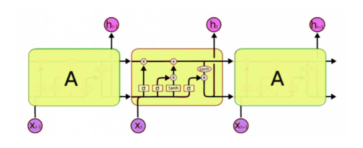
An LSTM will take the data through what it calls “cells” as you can see in the diagram above depicted in the middle rectangle. It is through this cell state that the LSTM can choose to remember or forget things.
An LSTM will have 3 different dependencies according to the information it receives:
To the domain of financial asset price prediction, these dependencies can be explained as below:
- The Previous Cell State – The trend of the stock on the previous day.
- The Previous Hidden State – The price of the stock on the previous day.
- The Input at the Current Time Step – Other factors that can affect the price. This will typically be news alerts that become available to investors throughout the day.

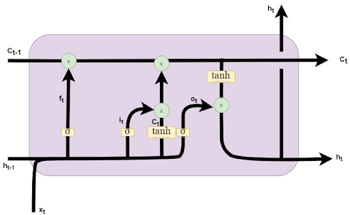
In the above diagram, the horizontal line ct denotes the cell state which is the memory of the LSTM. As we immediately mentioned above, this relates to the trend of the stock in the previous day (1). That information will flow into the cell and be processed with the other information that flows in. The line which is denoted by ct-1 is the Hidden State (2) which in our case of stock prediction will contain the previous time steps information (i.e. previous day’s stock price). The horizontal line denoted by ht-1 is the input at the current time which is the current stock price (3). Using the information from the previous stock price (Hidden State), the current price combined with the previous day’s trend (Cell State), the LSTM will generate an output.
Python Code to Create an LSTM Prediction Model
The following Python code takes us through steps to create an LSTM model predicting the price of a stock.
from google.colab import files
uploaded = files.upload()


import io
import pandas as pd
import numpy as np
import matplotlib.pyplot as plt
%matplotlib inline
from matplotlib.pylab import rcParams
rcParams['figure.figsize']=20,10
from keras.models import Sequential
from keras.layers import LSTM,Dropout,Dense
from sklearn.preprocessing import MinMaxScaler

df = pd.read_csv(io.BytesIO(uploaded['NSE-Tata-Global-Beverages-Limited.csv']))

print(df)

df["Date"]=pd.to_datetime(df.Date,format="%Y-%m-%d")
df.index=df['Date']


data=df.sort_index(ascending=True,axis=0)
new_dataset=pd.DataFrame(index=range(0,len(df)),columns=['Date','Close'])


for i in range(0,len(data)):
    new_dataset["Date"][i]=data['Date'][i]
    new_dataset["Close"][i]=data["Close"][i]

train_data=final_dataset[0:987,:]
valid_data=final_dataset[987:,:]

new_dataset.index=new_dataset.Date
new_dataset.drop("Date",axis=1,inplace=True)

scaler=MinMaxScaler(feature_range=(0,1))
scaled_data=scaler.fit_transform(new_dataset)

x_train_data,y_train_data=[],[]
for i in range(60,len(train_data)):
    x_train_data.append(scaled_data[i-60:i,0])
    y_train_data.append(scaled_data[i,0])

x_train_data,y_train_data=np.array(x_train_data),np.array(y_train_data)

x_train_data=np.reshape(x_train_data,(x_train_data.shape[0],x_train_data.shape[1],1))

lstm_model=Sequential()
lstm_model.add(LSTM(units=50,return_sequences=True,input_shape=(x_train_data.shape[1],1)))
lstm_model.add(LSTM(units=50))
lstm_model.add(Dense(1))

inputs_data=new_dataset[len(new_dataset)-len(valid_data)-60:].values
inputs_data=inputs_data.reshape(-1,1)
inputs_data=scaler.transform(inputs_data)

lstm_model.compile(loss='mean_squared_error',optimizer='adam')
lstm_model.fit(x_train_data,y_train_data,epochs=1,batch_size=1,verbose=2)

X_test=[]
for i in range(60,inputs_data.shape[0]):
    X_test.append(inputs_data[i-60:i,0])

X_test=np.array(X_test)

X_test=np.reshape(X_test,(X_test.shape[0],X_test.shape[1],1))

predicted_closing_price=lstm_model.predict(X_test)
predicted_closing_price=scaler.inverse_transform(predicted_closing_price)


train_data=new_dataset[:987]
valid_data=new_dataset[987:]
valid_data['Predictions']=predicted_closing_price
A Program Capable of Predicting Stock Market Prices Using LSTM
You now have the Python code to get you started predicting the prices of stock on the stock exchanges using LSTM. Give it a try and let us know how it works for you. We are just at the beginning of unpacking LSTM’s capability in different applications, and we are excited about the future.
Learn more about how LSTM Recurrent Neural Networks are being used in other applications.
Have any questions about deep learning workstations or servers?
Contact Exxact Today

Forecasting Stock Prices with LSTM–An Artificial Recurrent Neural Network (RNN)
How to Predict Stock Market Prices Using LSTM
The financial industry was one of the first industries to embrace the use of machine learning and deep learning in its investment analysis and operations to add value to their customers. Prior to machine learning, deep learning, and the entire “Quant” revolution in the 2000’s up until now, analysts and investors relied on less technologically reliant techniques. Fundamental and technical analysis reigned supreme and, although they still make up a big part of the analysis, they’re now combined with forecasts and analysis done by computers.
As most people know, the stock market is a place where people buy and sell stocks. The act of buying and selling these stocks (i.e. trading) takes place in physical and virtual environments called “Exchanges”. These exchanges are houses for indexes (commonly known ones are the Dow Jones Industrial Average and NASDAQ Composite). The exchanges are where the price of stocks that make up the indexes are set.
There are many factors that can fluctuate the price of a stock. Daily news reports bearing good or bad news about the current or future prospects of a company is arguably one of the most influential factors driving daily price fluctuations. A company’s profitability, revenue growth and future expansion prospects are indicators that can set long term and short term price changes. Deep Learning and other statistical models can only account for so much and is usually better suited for short-medium term forecasting rather than long term (e.g. years).
Interested in getting faster results?
Learn more about Exxact Deep Learning Solutions
Unpacking Long Short Term Memory Models (LSTM)

LSTM’s are a derivative of a Recurrent Neural Network (RNN). An RNN is an adequate model for a short time horizon of perhaps a week to a month. Going further than that the RNN is unlikely to produce reliable forecasts. This is due to the Vanishing Gradient Problem.
A normal time series method such as AR and its derivatives or ANN (Artificial Neural Network) may learn by applying a large weight towards the previous day’s price plus some other features. For Financial Time Series, you would use ARCH models and their derivatives to predict the returns or volatility. In a feed forward network, these points are considered as independent from each other. This means that the LSTM does not take the same approach as the traditional time series forecasting methods.
LSTM Uses Different Dependencies in Forecasting
An LSTM will take the data through what it calls “cells” as you can see in the diagram above depicted in the middle rectangle. It is through this cell state that the LSTM can choose to remember or forget things.
An LSTM will have 3 different dependencies according to the information it receives:
To the domain of financial asset price prediction, these dependencies can be explained as below:
- The Previous Cell State – The trend of the stock on the previous day.
- The Previous Hidden State – The price of the stock on the previous day.
- The Input at the Current Time Step – Other factors that can affect the price. This will typically be news alerts that become available to investors throughout the day.

In the above diagram, the horizontal line ct denotes the cell state which is the memory of the LSTM. As we immediately mentioned above, this relates to the trend of the stock in the previous day (1). That information will flow into the cell and be processed with the other information that flows in. The line which is denoted by ct-1 is the Hidden State (2) which in our case of stock prediction will contain the previous time steps information (i.e. previous day’s stock price). The horizontal line denoted by ht-1 is the input at the current time which is the current stock price (3). Using the information from the previous stock price (Hidden State), the current price combined with the previous day’s trend (Cell State), the LSTM will generate an output.
Python Code to Create an LSTM Prediction Model
The following Python code takes us through steps to create an LSTM model predicting the price of a stock.
from google.colab import files
uploaded = files.upload()


import io
import pandas as pd
import numpy as np
import matplotlib.pyplot as plt
%matplotlib inline
from matplotlib.pylab import rcParams
rcParams['figure.figsize']=20,10
from keras.models import Sequential
from keras.layers import LSTM,Dropout,Dense
from sklearn.preprocessing import MinMaxScaler

df = pd.read_csv(io.BytesIO(uploaded['NSE-Tata-Global-Beverages-Limited.csv']))

print(df)

df["Date"]=pd.to_datetime(df.Date,format="%Y-%m-%d")
df.index=df['Date']


data=df.sort_index(ascending=True,axis=0)
new_dataset=pd.DataFrame(index=range(0,len(df)),columns=['Date','Close'])


for i in range(0,len(data)):
    new_dataset["Date"][i]=data['Date'][i]
    new_dataset["Close"][i]=data["Close"][i]

train_data=final_dataset[0:987,:]
valid_data=final_dataset[987:,:]

new_dataset.index=new_dataset.Date
new_dataset.drop("Date",axis=1,inplace=True)

scaler=MinMaxScaler(feature_range=(0,1))
scaled_data=scaler.fit_transform(new_dataset)

x_train_data,y_train_data=[],[]
for i in range(60,len(train_data)):
    x_train_data.append(scaled_data[i-60:i,0])
    y_train_data.append(scaled_data[i,0])

x_train_data,y_train_data=np.array(x_train_data),np.array(y_train_data)

x_train_data=np.reshape(x_train_data,(x_train_data.shape[0],x_train_data.shape[1],1))

lstm_model=Sequential()
lstm_model.add(LSTM(units=50,return_sequences=True,input_shape=(x_train_data.shape[1],1)))
lstm_model.add(LSTM(units=50))
lstm_model.add(Dense(1))

inputs_data=new_dataset[len(new_dataset)-len(valid_data)-60:].values
inputs_data=inputs_data.reshape(-1,1)
inputs_data=scaler.transform(inputs_data)

lstm_model.compile(loss='mean_squared_error',optimizer='adam')
lstm_model.fit(x_train_data,y_train_data,epochs=1,batch_size=1,verbose=2)

X_test=[]
for i in range(60,inputs_data.shape[0]):
    X_test.append(inputs_data[i-60:i,0])

X_test=np.array(X_test)

X_test=np.reshape(X_test,(X_test.shape[0],X_test.shape[1],1))

predicted_closing_price=lstm_model.predict(X_test)
predicted_closing_price=scaler.inverse_transform(predicted_closing_price)


train_data=new_dataset[:987]
valid_data=new_dataset[987:]
valid_data['Predictions']=predicted_closing_price
A Program Capable of Predicting Stock Market Prices Using LSTM
You now have the Python code to get you started predicting the prices of stock on the stock exchanges using LSTM. Give it a try and let us know how it works for you. We are just at the beginning of unpacking LSTM’s capability in different applications, and we are excited about the future.
Learn more about how LSTM Recurrent Neural Networks are being used in other applications.
Have any questions about deep learning workstations or servers?
Contact Exxact Today


