What is Apache Spark?
Apache Spark is one of the hottest new trends in the technology domain. It is the framework with probably the highest potential to realize the fruit of the marriage between Big Data and Machine Learning.
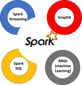
It runs fast (up to 100x faster than traditional Hadoop MapReduce due to in-memory operation, offers robust, distributed, fault-tolerant data objects (called RDD), and integrates beautifully with the world of machine learning and graph analytics through supplementary packages like Mlib and GraphX.
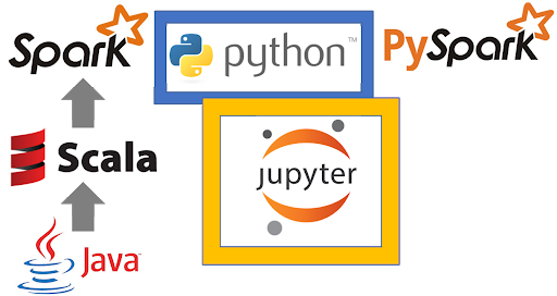
Spark is implemented on Hadoop/HDFS and written mostly in Scala, a functional programming language, similar to Java. In fact, Scala needs the latest Java installation on your system and runs on JVM. However, for most beginners, Scala is not a language that they learn first to venture into the world of data science. Fortunately, Spark provides a wonderful Python integration, called PySpark, which lets Python programmers to interface with the Spark framework and learn how to manipulate data at scale and work with objects and algorithms over a distributed file system.
In this article, we will learn the basics of PySpark. There are a lot of concepts (constantly evolving and introduced), and therefore, we just focus on fundamentals with a few simple examples. Readers are encouraged to build on these and explore more on their own.
The Short History of Apache Spark
Apache Spark started as a research project at the UC Berkeley AMPLab in 2009 and was open-sourced in early 2010. It was a class project at UC Berkeley. Idea was to build a cluster management framework, which can support different kinds of cluster computing systems. Many of the ideas behind the system were presented in various research papers over the years. After being released, Spark grew into a broad developer community and moved to the Apache Software Foundation in 2013. Today, the project is developed collaboratively by a community of hundreds of developers from hundreds of organizations.
Spark is Not a Programming Language
One thing to remember is that Spark is not a programming language like Python or Java. It is a general-purpose distributed data processing engine, suitable for use in a wide range of circumstances. It is particularly useful for big data processing both at scale and at high speed.
Application developers and data scientists generally incorporate Spark into their applications to rapidly query, analyze, and transform data at scale. Some of the tasks that are most frequently associated with Spark include, - ETL and SQL batch jobs across large data sets (often of terabytes of size), - processing of streaming data from IoT devices and nodes, data from various sensors, financial and transactional systems of all kinds, and - machine learning tasks for e-commerce or IT applications.
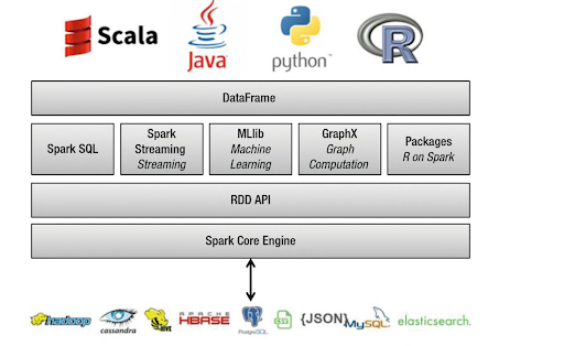
At its core, Spark builds on top of the Hadoop/HDFS framework for handling distributed files. It is mostly implemented with Scala, a functional language variant of Java. There is a core Spark data processing engine, but on top of that, there are many libraries developed for SQL-type query analysis, distributed machine learning, large-scale graph computation, and streaming data processing. Multiple programming languages are supported by Spark in the form of easy interface libraries: Java, Python, Scala, and R.
Spark Uses the MapReduce Paradigm for Distributed Processing
The basic idea of distributed processing is to divide the data chunks into small manageable pieces (including some filtering and sorting), bring the computation close to the data i.e. using small nodes of a large cluster for specific jobs and then re-combine them back. The dividing portion is called the ‘Map’ action and the recombination is called the ‘Reduce’ action. Together, they make the famous ‘MapReduce’ paradigm, which was introduced by Google around 2004 (see the original paper here).
For example, if a file has 100 records to be processed, 100 mappers can run together to process one record each. Or maybe 50 mappers can run together to process two records each. After all the mappers complete processing, the framework shuffles and sorts the results before passing them on to the reducers. A reducer cannot start while a mapper is still in progress. All the map output values that have the same key are assigned to a single reducer, which then aggregates the values for that key.

How to Setup PySpark
If you’re already familiar with Python and libraries such as Pandas and Numpy, then PySpark is a great extension/framework to learn in order to create more scalable, data-intensive analyses and pipelines by utilizing the power of Spark in the background.
The exact process of installing and setting up PySpark environment (on a standalone machine) is somewhat involved and can vary slightly depending on your system and environment. The goal is to get your regular Jupyter data science environment working with Spark in the background using the PySpark package.
This article on Medium provides more details on the step-by-step setup process.
Alternatively, you can use Databricks setup for practicing Spark. This company was created by the original creators of Spark and have an excellent ready-to-launch environment to do distributed analysis with Spark.
But the idea is always the same. You are distributing (and replicating) your large dataset in small fixed chunks over many nodes. You then bring the compute engine close to them so that the whole operation is parallelized, fault-tolerant and scalable.
By working with PySpark and Jupyter notebook, you can learn all these concepts without spending anything on AWS or Databricks platform. You can also easily interface with SparkSQL and MLlib for database manipulation and machine learning. It will be much easier to start working with real-life large clusters if you have internalized these concepts beforehand!
Resilient Distributed Dataset (RDD) and SparkContext
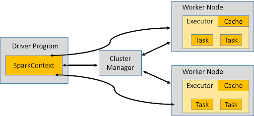
Many Spark programs revolve around the concept of a resilient distributed dataset (RDD), which is a fault-tolerant collection of elements that can be operated on in parallel. SparkContext resides in the Driver program and manages the distributed data over the worker nodes through the cluster manager. The good thing about using PySpark is that all this complexity of data partitioning and task management is handled automatically at the back and the programmer can focus on the specific analytics or machine learning job itself.
rdd-1
There are two ways to create RDDs–parallelizing an existing collection in your driver program or referencing a dataset in an external storage system, such as a shared file- system, HDFS, HBase, or any data source offering a Hadoop InputFormat.
For illustration with a Python-based approach, we will give examples of the first type here. We can create a simple Python array of 20 random integers (between 0 and 10), using Numpy random.randint(), and then create an RDD object as following,
from pyspark import SparkContext
import numpy as np
sc=SparkContext(master="local[4]")
lst=np.random.randint(0,10,20)
A=sc.parallelize(lst)
Note the ‘4’ in the argument. It denotes 4 computing cores (in your local machine) to be used for this SparkContext object. If we check the type of the RDD object, we get the following,
type(A)
>> pyspark.rdd.RDD
Opposite to parallelization is the collection (with collect()) which brings all the distributed elements and returns them to the head node.
A.collect()
>> [4, 8, 2, 2, 4, 7, 0, 3, 3, 9, 2, 6, 0, 0, 1, 7, 5, 1, 9, 7]
But A is no longer a simple Numpy array. We can use the glom() method to check how the partitions are created.
A.glom().collect()
>> [[4, 8, 2, 2, 4], [7, 0, 3, 3, 9], [2, 6, 0, 0, 1], [7, 5, 1, 9, 7]]
Now stop the SC and reinitialize it with 2 cores and see what happens when you repeat the process.
sc.stop()
sc=SparkContext(master="local[2]")
A = sc.parallelize(lst)
A.glom().collect()
>> [[4, 8, 2, 2, 4, 7, 0, 3, 3, 9], [2, 6, 0, 0, 1, 7, 5, 1, 9, 7]]
The RDD is now distributed over two chunks, not four!
You have learned about the first step in distributed data analytics i.e. controlling how your data is partitioned over smaller chunks for further processing
Some Examples of Basic Operations with RDD & PySpark
Count the elements
>> 20
The first element (first) and the first few elements (take)
A.first()
>> 4
A.take(3)
>> [4, 8, 2]
Removing duplicates with using distinct
NOTE: This operation requires a shuffle in order to detect duplication across partitions. So, it is a slow operation. Don’t overdo it.
A_distinct=A.distinct()
A_distinct.collect()
>> [4, 8, 0, 9, 1, 5, 2, 6, 7, 3]
To sum, all the elements use the reduce method
Note the use of a lambda function in this,
A.reduce(lambda x,y:x+y)
>> 80
Or the direct sum() method
A.sum()
>> 80
Finding maximum element by reducing
A.reduce(lambda x,y: x if x > y else y)
>> 9
Finding the longest word in a blob of text
words = 'These are some of the best Macintosh computers ever'.split(' ')
wordRDD = sc.parallelize(words)
wordRDD.reduce(lambda w,v: w if len(w)>len(v) else v)
>> 'computers'
Use the filter for logic-based filtering
# Return RDD with elements (greater than zero) divisible by 3
A.filter(lambda x:x%3==0 and x!=0).collect()
>> [3, 3, 9, 6, 9]
Write regular Python functions to use with reduce()
def largerThan(x,y):
    """
    Returns the last word among the longest words in a list
    """
    if len(x)> len(y):
        return x
    elif len(y) > len(x):
        return y
    else:
        if x < y: return x
        else: return y

wordRDD.reduce(largerThan)
>> 'Macintosh'
Note here the x < y does a lexicographic comparison and determines that Macintosh is larger than computers!
Mapping operation with a lambda function with PySpark
B=A.map(lambda x:x*x)
B.collect()
>> [16, 64, 4, 4, 16, 49, 0, 9, 9, 81, 4, 36, 0, 0, 1, 49, 25, 1, 81, 49]
Mapping with a regular Python function in PySpark
def square_if_odd(x):
    """
    Squares if odd, otherwise keeps the argument unchanged
    """
    if x%2==1:
        return x*x
    else:
        return x

A.map(square_if_odd).collect()
>> [4, 8, 2, 2, 4, 49, 0, 9, 9, 81, 2, 6, 0, 0, 1, 49, 25, 1, 81, 49]
groupby returns an RDD of grouped elements (iterable) as per a given group operation
In the following example, we use a list-comprehension along with the group to create a list of two elements, each having a header (the result of the lambda function, simple modulo 2 here), and a sorted list of the elements which gave rise to that result. You can imagine easily that this kind of separation can come particularly handy for processing data which needs to be binned/canned out based on particular operation performed over them.
result=A.groupBy(lambda x:x%2).collect()
sorted([(x, sorted(y)) for (x, y) in result])
>> [(0, [0, 0, 0, 2, 2, 2, 4, 4, 6, 8]), (1, [1, 1, 3, 3, 5, 7, 7, 7, 9, 9])]
Using histogram
The histogram() method takes a list of bins/buckets and returns a tuple with the result of the histogram (binning),
B.histogram([x for x in range(0,100,10)])
>> ([0, 10, 20, 30, 40, 50, 60, 70, 80, 90], [10, 2, 1, 1, 3, 0, 1, 0, 2])
Set operations
You can also do regular set operations on RDDs like - union(), intersection(), subtract(), or cartesian().
Check out this Jupyter notebook for more examples.

Lazy evaluation with PySpark (and Caching)
Lazy evaluation is an evaluation/computation strategy which prepares a detailed step-by-step internal map of the execution pipeline for a computing task but delays the final execution until when it is absolutely needed. This strategy is at the heart of Spark for speeding up many parallelized Big Data operations.
Let’s use two CPU cores for this example,
sc = SparkContext(master="local[2]")
Make a RDD with 1 million elements
%%time
rdd1 = sc.parallelize(range(1000000))
>> CPU times: user 316 µs, sys: 5.13 ms, total: 5.45 ms, Wall time: 24.6 ms
Some computing function – taketime
from math import cos
def taketime(x):
    [cos(j) for j in range(100)]
    return cos(x)
Check how much time is taken by taketime function
%%time
taketime(2)
>> CPU times: user 21 µs, sys: 7 µs, total: 28 µs, Wall time: 31.5 µs
>> -0.4161468365471424
Remember this result, the taketime() function took a wall time of 31.5 us. Of course, the exact number will depend on the machine you are working on.
Now do the map operation on the function
%%time
interim = rdd1.map(lambda x: taketime(x))
>> CPU times: user 23 µs, sys: 8 µs, total: 31 µs, Wall time: 34.8 µs
How come each taketime function takes 45.8 us but the map operation with a 1 million elements RDD also took a similar time?
Because of lazy evaluation i.e., nothing was computed in the previous step, just a plan of execution was made. The variable interim does not point to a data structure, instead, it points to a plan of execution, expressed as a dependency graph. The dependency graph defines how RDDs are computed from each other.
The actual execution by reducing method
%%time
print('output =',interim.reduce(lambda x,y:x+y))
>> output = -0.28870546796843666
>> CPU times: user 11.6 ms, sys: 5.56 ms, total: 17.2 ms, Wall time: 15.6 s
So, the wall time here is 15.6 seconds. Remember, the taketime() function had a wall time of 31.5 us? Therefore, we expect the total time to be on the order of ~ 31 seconds for a 1-million array. Because of parallel operation on two cores, it took ~ 15 seconds.
Now, we have not saved (materialized) any intermediate results in the interim, so another simple operation (e.g. counting elements > 0) will take the almost the same time.
%%time
print(interim.filter(lambda x:x>0).count())
>> 500000
>> CPU times: user 10.6 ms, sys: 8.55 ms, total: 19.2 ms, Wall time: 12.1 s
Caching to reduce computation time on similar operation (spending memory)
Remember the dependency graph that we built in the previous step? We can run the same computation as before with cache method to tell the dependency graph to plan for caching.
%%time
interim = rdd1.map(lambda x: taketime(x)).cache()
The first computation will not improve, but it caches the interim result,
%%time
print('output =',interim.reduce(lambda x,y:x+y))
>> output = -0.28870546796843666
>> CPU times: user 16.4 ms, sys: 2.24 ms, total: 18.7 ms, Wall time: 15.3 s
Now run the same filter method with the help of cached result,
%%time
print(interim.filter(lambda x:x>0).count())
>> 500000
>> CPU times: user 14.2 ms, sys: 3.27 ms, total: 17.4 ms, Wall time: 811 ms
Wow! The computing time came down to less than a second from 12 seconds earlier! This way, caching and parallelization with lazy execution, is the core feature of programming with Spark.
Dataframe and SparkSQL
Apart from the RDD, the second key data structure in the Spark framework is the DataFrame. If you have done work with Python Pandas or R DataFrame, the concept may seem familiar.
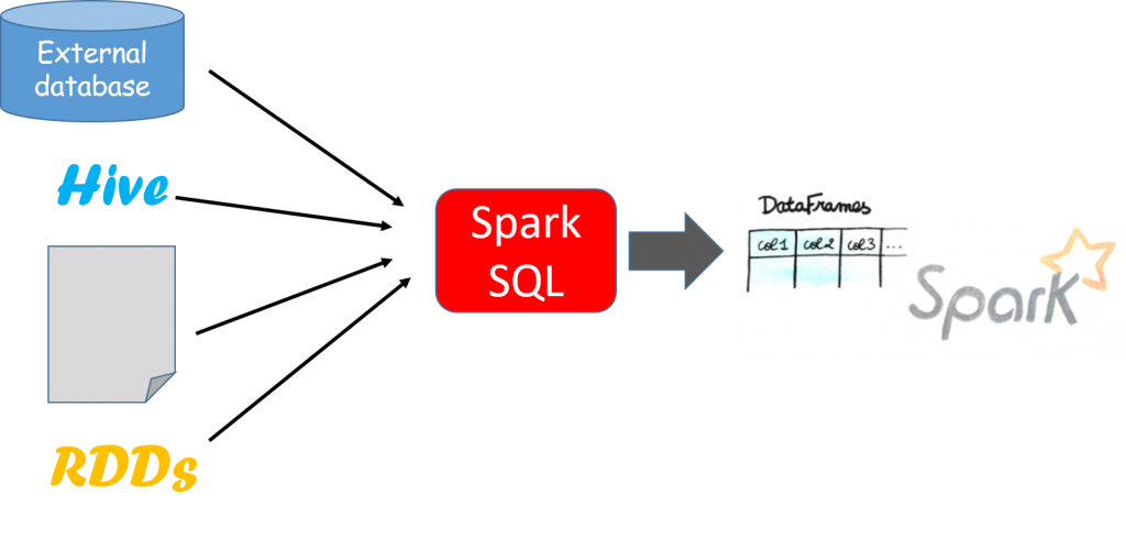
A DataFrame is a distributed collection of rows under named columns. It is conceptually equivalent to a table in a relational database, an Excel sheet with Column headers, or a data frame in R/Python, but with richer optimizations under the hood. DataFrames can be constructed from a wide array of sources such as structured data files, tables in Hive, external databases, or existing RDDs. It also shares some common characteristics with RDD:
- Immutable in nature: We can create DataFrame / RDD once but can’t change it. And we can transform a DataFrame / RDD after applying transformations.
- Lazy Evaluations: This means that a task is not executed until an action is performed. Distributed: RDD and DataFrame both are distributed in nature.
Advantages of the DataFrame
- DataFrames are designed for processing a large collection of structured or semi-structured data.
- Observations in Spark DataFrame are organized under named columns, which helps Apache Spark to understand the schema of a DataFrame. This helps Spark optimize the execution plan on these queries.
- DataFrame in Apache Spark has the ability to handle petabytes of data.
- DataFrame has support for a wide range of data formats and sources.
- It has API support for different languages like Python, R, Scala, Java.
SparkSQL Helps to Bridge the Gap for PySpark
Relational data stores are easy to build and query. Users and developers often prefer writing easy-to-interpret, declarative queries in a human-like readable language such as SQL. However, as data starts increasing in volume and variety, the relational approach does not scale well enough for building Big Data applications and analytical systems.
We have had success in the domain of Big Data analytics with Hadoop and the MapReduce paradigm. This was powerful, but often slow, and gave users a low-level, procedural programming interface that required people to write a lot of code for even very simple data transformations. However, once Spark was released, it really revolutionized the way Big Data analytics was done with a focus on in-memory computing, fault tolerance, high-level abstractions, and ease of use.
Spark SQL essentially tries to bridge the gap between the two models we mentioned previously—the relational and procedural models. Spark SQL works through the DataFrame API that can perform relational operations on both external data sources and Spark’s built-in distributed collections—at scale!
Why is Spark SQL so fast and optimized? The reason is because of a new extensible optimizer, Catalyst, based on functional programming constructs in Scala. Catalyst supports both rule-based and cost-based optimization. While extensible optimizers have been proposed in the past, they have typically required a complex domain-specific language to specify rules. Usually, this leads to having a significant learning curve and maintenance burden. In contrast, Catalyst uses standard features of the Scala programming language, such as pattern-matching, to let developers use the full programming language while still making rules easy to specify.
You can refer to the following Jupyter notebook for an introduction to Database operations with SparkSQL:
SparkSQL database operations basics
How Are You Going to Use PySpark in Your Project?
We covered the fundamentals of the Apache Spark ecosystem and how it works along with some basic usage examples of core data structure RDD with the Python interface PySpark. Also, DataFrame and SparkSQL were discussed along with reference links for example code notebooks.
There is so much more to learn and experiment with Apache Spark being used with Python. The PySpark website is a good reference to have on your radar, and they make regular updates and enhancements–so keep an eye on that.
And, if you are interested in doing large-scale, distributed machine learning with Apache Spark, then check out the MLLib portion of the PySpark ecosystem.
Did you Enjoy This PySpark Blog? Be Sure to Check Out:


The Benefits & Examples of Using Apache Spark with PySpark
What is Apache Spark?
Apache Spark is one of the hottest new trends in the technology domain. It is the framework with probably the highest potential to realize the fruit of the marriage between Big Data and Machine Learning.
It runs fast (up to 100x faster than traditional Hadoop MapReduce due to in-memory operation, offers robust, distributed, fault-tolerant data objects (called RDD), and integrates beautifully with the world of machine learning and graph analytics through supplementary packages like Mlib and GraphX.

Spark is implemented on Hadoop/HDFS and written mostly in Scala, a functional programming language, similar to Java. In fact, Scala needs the latest Java installation on your system and runs on JVM. However, for most beginners, Scala is not a language that they learn first to venture into the world of data science. Fortunately, Spark provides a wonderful Python integration, called PySpark, which lets Python programmers to interface with the Spark framework and learn how to manipulate data at scale and work with objects and algorithms over a distributed file system.
In this article, we will learn the basics of PySpark. There are a lot of concepts (constantly evolving and introduced), and therefore, we just focus on fundamentals with a few simple examples. Readers are encouraged to build on these and explore more on their own.
The Short History of Apache Spark
Apache Spark started as a research project at the UC Berkeley AMPLab in 2009 and was open-sourced in early 2010. It was a class project at UC Berkeley. Idea was to build a cluster management framework, which can support different kinds of cluster computing systems. Many of the ideas behind the system were presented in various research papers over the years. After being released, Spark grew into a broad developer community and moved to the Apache Software Foundation in 2013. Today, the project is developed collaboratively by a community of hundreds of developers from hundreds of organizations.
Spark is Not a Programming Language
One thing to remember is that Spark is not a programming language like Python or Java. It is a general-purpose distributed data processing engine, suitable for use in a wide range of circumstances. It is particularly useful for big data processing both at scale and at high speed.
Application developers and data scientists generally incorporate Spark into their applications to rapidly query, analyze, and transform data at scale. Some of the tasks that are most frequently associated with Spark include, - ETL and SQL batch jobs across large data sets (often of terabytes of size), - processing of streaming data from IoT devices and nodes, data from various sensors, financial and transactional systems of all kinds, and - machine learning tasks for e-commerce or IT applications.
At its core, Spark builds on top of the Hadoop/HDFS framework for handling distributed files. It is mostly implemented with Scala, a functional language variant of Java. There is a core Spark data processing engine, but on top of that, there are many libraries developed for SQL-type query analysis, distributed machine learning, large-scale graph computation, and streaming data processing. Multiple programming languages are supported by Spark in the form of easy interface libraries: Java, Python, Scala, and R.
Spark Uses the MapReduce Paradigm for Distributed Processing
The basic idea of distributed processing is to divide the data chunks into small manageable pieces (including some filtering and sorting), bring the computation close to the data i.e. using small nodes of a large cluster for specific jobs and then re-combine them back. The dividing portion is called the ‘Map’ action and the recombination is called the ‘Reduce’ action. Together, they make the famous ‘MapReduce’ paradigm, which was introduced by Google around 2004 (see the original paper here).
For example, if a file has 100 records to be processed, 100 mappers can run together to process one record each. Or maybe 50 mappers can run together to process two records each. After all the mappers complete processing, the framework shuffles and sorts the results before passing them on to the reducers. A reducer cannot start while a mapper is still in progress. All the map output values that have the same key are assigned to a single reducer, which then aggregates the values for that key.

How to Setup PySpark
If you’re already familiar with Python and libraries such as Pandas and Numpy, then PySpark is a great extension/framework to learn in order to create more scalable, data-intensive analyses and pipelines by utilizing the power of Spark in the background.
The exact process of installing and setting up PySpark environment (on a standalone machine) is somewhat involved and can vary slightly depending on your system and environment. The goal is to get your regular Jupyter data science environment working with Spark in the background using the PySpark package.
This article on Medium provides more details on the step-by-step setup process.

Alternatively, you can use Databricks setup for practicing Spark. This company was created by the original creators of Spark and have an excellent ready-to-launch environment to do distributed analysis with Spark.
But the idea is always the same. You are distributing (and replicating) your large dataset in small fixed chunks over many nodes. You then bring the compute engine close to them so that the whole operation is parallelized, fault-tolerant and scalable.
By working with PySpark and Jupyter notebook, you can learn all these concepts without spending anything on AWS or Databricks platform. You can also easily interface with SparkSQL and MLlib for database manipulation and machine learning. It will be much easier to start working with real-life large clusters if you have internalized these concepts beforehand!
Resilient Distributed Dataset (RDD) and SparkContext
Many Spark programs revolve around the concept of a resilient distributed dataset (RDD), which is a fault-tolerant collection of elements that can be operated on in parallel. SparkContext resides in the Driver program and manages the distributed data over the worker nodes through the cluster manager. The good thing about using PySpark is that all this complexity of data partitioning and task management is handled automatically at the back and the programmer can focus on the specific analytics or machine learning job itself.

rdd-1
There are two ways to create RDDs–parallelizing an existing collection in your driver program or referencing a dataset in an external storage system, such as a shared file- system, HDFS, HBase, or any data source offering a Hadoop InputFormat.
For illustration with a Python-based approach, we will give examples of the first type here. We can create a simple Python array of 20 random integers (between 0 and 10), using Numpy random.randint(), and then create an RDD object as following,
from pyspark import SparkContext
import numpy as np
sc=SparkContext(master="local[4]")
lst=np.random.randint(0,10,20)
A=sc.parallelize(lst)
Note the ‘4’ in the argument. It denotes 4 computing cores (in your local machine) to be used for this SparkContext object. If we check the type of the RDD object, we get the following,
type(A)
>> pyspark.rdd.RDD
Opposite to parallelization is the collection (with collect()) which brings all the distributed elements and returns them to the head node.
A.collect()
>> [4, 8, 2, 2, 4, 7, 0, 3, 3, 9, 2, 6, 0, 0, 1, 7, 5, 1, 9, 7]
But A is no longer a simple Numpy array. We can use the glom() method to check how the partitions are created.
A.glom().collect()
>> [[4, 8, 2, 2, 4], [7, 0, 3, 3, 9], [2, 6, 0, 0, 1], [7, 5, 1, 9, 7]]
Now stop the SC and reinitialize it with 2 cores and see what happens when you repeat the process.
sc.stop()
sc=SparkContext(master="local[2]")
A = sc.parallelize(lst)
A.glom().collect()
>> [[4, 8, 2, 2, 4, 7, 0, 3, 3, 9], [2, 6, 0, 0, 1, 7, 5, 1, 9, 7]]
The RDD is now distributed over two chunks, not four!
You have learned about the first step in distributed data analytics i.e. controlling how your data is partitioned over smaller chunks for further processing
Some Examples of Basic Operations with RDD & PySpark
Count the elements
>> 20
The first element (first) and the first few elements (take)
A.first()
>> 4
A.take(3)
>> [4, 8, 2]
Removing duplicates with using distinct
NOTE: This operation requires a shuffle in order to detect duplication across partitions. So, it is a slow operation. Don’t overdo it.
A_distinct=A.distinct()
A_distinct.collect()
>> [4, 8, 0, 9, 1, 5, 2, 6, 7, 3]
To sum, all the elements use the reduce method
Note the use of a lambda function in this,
A.reduce(lambda x,y:x+y)
>> 80
Or the direct sum() method
A.sum()
>> 80
Finding maximum element by reducing
A.reduce(lambda x,y: x if x > y else y)
>> 9
Finding the longest word in a blob of text
words = 'These are some of the best Macintosh computers ever'.split(' ')
wordRDD = sc.parallelize(words)
wordRDD.reduce(lambda w,v: w if len(w)>len(v) else v)
>> 'computers'
Use the filter for logic-based filtering
# Return RDD with elements (greater than zero) divisible by 3
A.filter(lambda x:x%3==0 and x!=0).collect()
>> [3, 3, 9, 6, 9]
Write regular Python functions to use with reduce()
def largerThan(x,y):
    """
    Returns the last word among the longest words in a list
    """
    if len(x)> len(y):
        return x
    elif len(y) > len(x):
        return y
    else:
        if x < y: return x
        else: return y

wordRDD.reduce(largerThan)
>> 'Macintosh'
Note here the x < y does a lexicographic comparison and determines that Macintosh is larger than computers!
Mapping operation with a lambda function with PySpark
B=A.map(lambda x:x*x)
B.collect()
>> [16, 64, 4, 4, 16, 49, 0, 9, 9, 81, 4, 36, 0, 0, 1, 49, 25, 1, 81, 49]
Mapping with a regular Python function in PySpark
def square_if_odd(x):
    """
    Squares if odd, otherwise keeps the argument unchanged
    """
    if x%2==1:
        return x*x
    else:
        return x

A.map(square_if_odd).collect()
>> [4, 8, 2, 2, 4, 49, 0, 9, 9, 81, 2, 6, 0, 0, 1, 49, 25, 1, 81, 49]
groupby returns an RDD of grouped elements (iterable) as per a given group operation
In the following example, we use a list-comprehension along with the group to create a list of two elements, each having a header (the result of the lambda function, simple modulo 2 here), and a sorted list of the elements which gave rise to that result. You can imagine easily that this kind of separation can come particularly handy for processing data which needs to be binned/canned out based on particular operation performed over them.
result=A.groupBy(lambda x:x%2).collect()
sorted([(x, sorted(y)) for (x, y) in result])
>> [(0, [0, 0, 0, 2, 2, 2, 4, 4, 6, 8]), (1, [1, 1, 3, 3, 5, 7, 7, 7, 9, 9])]
Using histogram
The histogram() method takes a list of bins/buckets and returns a tuple with the result of the histogram (binning),
B.histogram([x for x in range(0,100,10)])
>> ([0, 10, 20, 30, 40, 50, 60, 70, 80, 90], [10, 2, 1, 1, 3, 0, 1, 0, 2])
Set operations
You can also do regular set operations on RDDs like - union(), intersection(), subtract(), or cartesian().
Check out this Jupyter notebook for more examples.

Lazy evaluation with PySpark (and Caching)
Lazy evaluation is an evaluation/computation strategy which prepares a detailed step-by-step internal map of the execution pipeline for a computing task but delays the final execution until when it is absolutely needed. This strategy is at the heart of Spark for speeding up many parallelized Big Data operations.
Let’s use two CPU cores for this example,
sc = SparkContext(master="local[2]")
Make a RDD with 1 million elements
%%time
rdd1 = sc.parallelize(range(1000000))
>> CPU times: user 316 µs, sys: 5.13 ms, total: 5.45 ms, Wall time: 24.6 ms
Some computing function – taketime
from math import cos
def taketime(x):
    [cos(j) for j in range(100)]
    return cos(x)
Check how much time is taken by taketime function
%%time
taketime(2)
>> CPU times: user 21 µs, sys: 7 µs, total: 28 µs, Wall time: 31.5 µs
>> -0.4161468365471424
Remember this result, the taketime() function took a wall time of 31.5 us. Of course, the exact number will depend on the machine you are working on.
Now do the map operation on the function
%%time
interim = rdd1.map(lambda x: taketime(x))
>> CPU times: user 23 µs, sys: 8 µs, total: 31 µs, Wall time: 34.8 µs
How come each taketime function takes 45.8 us but the map operation with a 1 million elements RDD also took a similar time?
Because of lazy evaluation i.e., nothing was computed in the previous step, just a plan of execution was made. The variable interim does not point to a data structure, instead, it points to a plan of execution, expressed as a dependency graph. The dependency graph defines how RDDs are computed from each other.
The actual execution by reducing method
%%time
print('output =',interim.reduce(lambda x,y:x+y))
>> output = -0.28870546796843666
>> CPU times: user 11.6 ms, sys: 5.56 ms, total: 17.2 ms, Wall time: 15.6 s
So, the wall time here is 15.6 seconds. Remember, the taketime() function had a wall time of 31.5 us? Therefore, we expect the total time to be on the order of ~ 31 seconds for a 1-million array. Because of parallel operation on two cores, it took ~ 15 seconds.
Now, we have not saved (materialized) any intermediate results in the interim, so another simple operation (e.g. counting elements > 0) will take the almost the same time.
%%time
print(interim.filter(lambda x:x>0).count())
>> 500000
>> CPU times: user 10.6 ms, sys: 8.55 ms, total: 19.2 ms, Wall time: 12.1 s
Caching to reduce computation time on similar operation (spending memory)
Remember the dependency graph that we built in the previous step? We can run the same computation as before with cache method to tell the dependency graph to plan for caching.
%%time
interim = rdd1.map(lambda x: taketime(x)).cache()
The first computation will not improve, but it caches the interim result,
%%time
print('output =',interim.reduce(lambda x,y:x+y))
>> output = -0.28870546796843666
>> CPU times: user 16.4 ms, sys: 2.24 ms, total: 18.7 ms, Wall time: 15.3 s
Now run the same filter method with the help of cached result,
%%time
print(interim.filter(lambda x:x>0).count())
>> 500000
>> CPU times: user 14.2 ms, sys: 3.27 ms, total: 17.4 ms, Wall time: 811 ms
Wow! The computing time came down to less than a second from 12 seconds earlier! This way, caching and parallelization with lazy execution, is the core feature of programming with Spark.
Dataframe and SparkSQL
Apart from the RDD, the second key data structure in the Spark framework is the DataFrame. If you have done work with Python Pandas or R DataFrame, the concept may seem familiar.
A DataFrame is a distributed collection of rows under named columns. It is conceptually equivalent to a table in a relational database, an Excel sheet with Column headers, or a data frame in R/Python, but with richer optimizations under the hood. DataFrames can be constructed from a wide array of sources such as structured data files, tables in Hive, external databases, or existing RDDs. It also shares some common characteristics with RDD:
- Immutable in nature: We can create DataFrame / RDD once but can’t change it. And we can transform a DataFrame / RDD after applying transformations.
- Lazy Evaluations: This means that a task is not executed until an action is performed. Distributed: RDD and DataFrame both are distributed in nature.

Advantages of the DataFrame
- DataFrames are designed for processing a large collection of structured or semi-structured data.
- Observations in Spark DataFrame are organized under named columns, which helps Apache Spark to understand the schema of a DataFrame. This helps Spark optimize the execution plan on these queries.
- DataFrame in Apache Spark has the ability to handle petabytes of data.
- DataFrame has support for a wide range of data formats and sources.
- It has API support for different languages like Python, R, Scala, Java.
SparkSQL Helps to Bridge the Gap for PySpark
Relational data stores are easy to build and query. Users and developers often prefer writing easy-to-interpret, declarative queries in a human-like readable language such as SQL. However, as data starts increasing in volume and variety, the relational approach does not scale well enough for building Big Data applications and analytical systems.
We have had success in the domain of Big Data analytics with Hadoop and the MapReduce paradigm. This was powerful, but often slow, and gave users a low-level, procedural programming interface that required people to write a lot of code for even very simple data transformations. However, once Spark was released, it really revolutionized the way Big Data analytics was done with a focus on in-memory computing, fault tolerance, high-level abstractions, and ease of use.
Spark SQL essentially tries to bridge the gap between the two models we mentioned previously—the relational and procedural models. Spark SQL works through the DataFrame API that can perform relational operations on both external data sources and Spark’s built-in distributed collections—at scale!

Why is Spark SQL so fast and optimized? The reason is because of a new extensible optimizer, Catalyst, based on functional programming constructs in Scala. Catalyst supports both rule-based and cost-based optimization. While extensible optimizers have been proposed in the past, they have typically required a complex domain-specific language to specify rules. Usually, this leads to having a significant learning curve and maintenance burden. In contrast, Catalyst uses standard features of the Scala programming language, such as pattern-matching, to let developers use the full programming language while still making rules easy to specify.
You can refer to the following Jupyter notebook for an introduction to Database operations with SparkSQL:
SparkSQL database operations basics
How Are You Going to Use PySpark in Your Project?
We covered the fundamentals of the Apache Spark ecosystem and how it works along with some basic usage examples of core data structure RDD with the Python interface PySpark. Also, DataFrame and SparkSQL were discussed along with reference links for example code notebooks.
There is so much more to learn and experiment with Apache Spark being used with Python. The PySpark website is a good reference to have on your radar, and they make regular updates and enhancements–so keep an eye on that.
And, if you are interested in doing large-scale, distributed machine learning with Apache Spark, then check out the MLLib portion of the PySpark ecosystem.
Did you Enjoy This PySpark Blog? Be Sure to Check Out:


