Artificial Intelligence for the Average User
Artificial intelligence (A.I.) is shaping up to be the most powerful and transformative technology to sweep the globe and touch all facets of life - economics, healthcare, finance, industry, socio-cultural interactions, etc. - in an unprecedented manner. This is even more important with developments in transfer learning and machine learning capabilities.
Already, we are using A.I. technologies on a daily basis, and it is impacting our lives and choices whether we consciously know it or not. From our Google search and Navigation, Netflix movie recommendations, Amazon purchase suggestions, voice assistants for daily tasks like Siri or Alexa, Facebook community building, medical diagnoses, credit score calculations, and mortgage decision making, etc., A.I. is only going to grow in adoption.
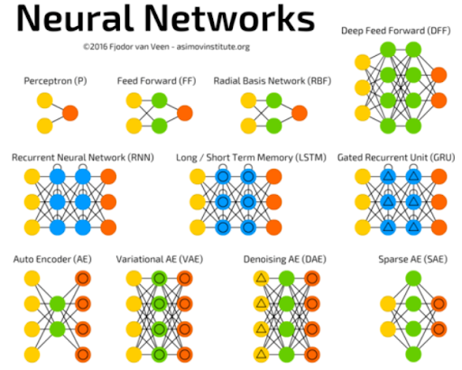
Most modern A.I. systems are currently being powered by a family of algorithms or techniques called deep learning, which basically trains and builds deep layers of neural networks with various architectural configurations.
Image source: Fjodor van Veen - asimovinstitute.org
After 50+ years of ebbs and flows, the deep learning revolution has caught the steam and looks unstoppable - fueled by Big Data technologies, innovation in hardware, and algorithms. Therefore, deep learning networks are promising to impact and fundamentally alter how we, humans, live, work, and play for at least the next few decades to come.
So, we can finally see the promise of A.I. for everyone on the planet!
However...there is a catch.
Deep Learning is Expensive and the Focus is Narrow
Deep learning networks tend to be resource-hungry and computationally expensive. Unlike traditional statistical learning models (such as regression, decision trees, or support vector machines), they tend to contain millions of parameters and therefore need a lot of training data to avoid overfitting.
Therefore, deep learning models are trained with massive amounts of high-dimensional raw data such as images, unstructured text, or audio signals. Also, they employ millions of vectorized computation (e.g. matrix multiplication) over and over, to optimize the huge parameter set to fit the data. Moreover, they are built with a large number of hyperparameters (e.g. number of layers, neurons per layer, optimizer algorithm settings, etc.) and it often takes many weeks or months for a team of highly trained researchers to create a state-of-the-art model.
All of these lead to a great demand on the computational power needed to train and robust and high-performance deep learning model, optimized for a given task.
Let’s say we can afford to train a great model after spending a huge amount of computational resources. Don’t we want to re-use this model for the maximum number and variety of tasks and reap the benefit of our investment many times over?
Herein lies the problem.
Deep learning algorithms, so far, have been traditionally designed to work in isolation. These algorithms are trained to solve specific tasks. The models, in most cases, have to be rebuilt from scratch once the feature-space distribution changes.
But, this does not make sense, especially when it is compared to how we humans currently utilize our limited computation speed.
Humans have an inherent ability to transfer knowledge across tasks. What we acquire as knowledge while learning about one task, we utilize in the same way to solve related tasks. If the similarity between the tasks or domains is high, we are able to cross-utilize our ‘learned’ knowledge better.
Transfer learning is the idea of overcoming the isolated learning paradigms and utilizing knowledge acquired for one task to solve related ones, as applied to machine learning, and in particular, to the domain of deep learning.
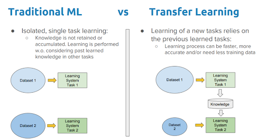
Image source: A Comprehensive Hands-on Guide to Transfer Learning with Real-World Applications in Deep Learning
Transfer Learning for Deep Learning Networks
There is a myriad of strategies to follow for the transfer learning process in the deep learning setting, and multiple important things to consider and engineering decisions to make - similarity of datasets and domains, supervised or unsupervised setting, how much retraining to be done, etc.
However, to put it very simply, we can assume that for transfer learning:
- We need to take a pre-trained deep learning model
- Re-use all or certain portions of it
- Apply it to our new domain of interest, for a particular machine learning problem–classification or regression.
In this way, we are able to avoid a large portion of the huge computational effort of training and optimizing a large deep learning model.
In the end, a trained deep learning model is just a collection of millions of real numbers in a particular data structure format, which can be used readily for prediction/inference, the task we are really interested in, as the consumers of the model.
But remember that a pre-trained model might have been trained using a particular classification in mind i.e. its output vector and computation graph is suited for the prediction of a particular task only.
Therefore, a widely used strategy in transfer learning is to:
- Load the weights matrices of a pre-trained model except for the weights of the very last layers near the O/P,
- Hold those weights fixed i.e. untrainable
- Attach new layers suitable for the task at hand, and train the model with new data
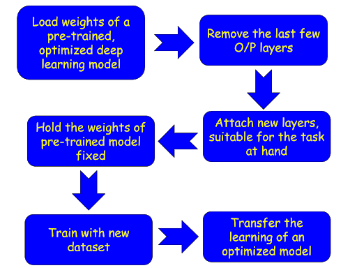
Fig: The transfer learning strategy for deep learning networks, as we will explore here.
This way, we don’t have to train the whole model, we get to repurpose the model for our specific machine learning task, yet can leverage the learned structures and patterns of the data, contained in the fixed weights, which are loaded from the pre-trained, optimized model.
A Hands-On Example You Can Run on Your Laptop
Let’s get our hands dirty and build a simple code demo to demonstrate the power of transfer learning, shall we?
Why not follow a traditional approach?
Now, traditionally, tutorials on this topic have focused on learning from famous, high-performance deep learning networks, such as VGGNet-16, ResNet-50, or Inception-V3/V4, etc. These networks were trained on the massive ImageNet database, and secured top places in the annual ImageNet competition - ILSVRC, thereby positioning themselves as the golden benchmark models for image classification tasks.
However, the issue with these networks, is that they contain a large number of complex layers, and not easy to understand when you are starting to learn deep learning concepts.
Therefore, if you want to code up a transfer learning example from scratch, it may be beneficial, from self-learning and confidence-building point of view, to try an independent example first. You can train a deep learning model first, transfer its learning to another seed network, and then show the performance on a standard classification task.
What are we going to do in this tutorial?
In this article, we will demonstrate the transfer learning concept in a very simple setting using Python, working with the Keras package (TensorFlow backend). We will take the well-known CIFAR-10 dataset and do the following:
- Create a Keras neural net by stacking a set of classificiation_layers on top of a set of feature_layers
- Train the resulting network on a partial CIFAR-10 dataset, consisting of examples from the first 5 categories (0...4).
- Freeze the feature_layers and stack a new set of fully-connected layers on top of them, thereby creating another conv net
- Train this new conv net on the examples from the rest of the categories (5..9) of CIFAR-10, tuning weights only for those densely connected layers
The entire code is open-source and can be found here. We show only some essential parts of the code here in this article.
Code Along
We start by importing the necessary libraries and functions:
from time import time
import keras
from keras.datasets import mnist,cifar10
from keras.models import Sequential
from keras.layers import Dense, Dropout, Activation, Flatten
from keras.layers import Conv2D, MaxPooling2D
from keras.optimizers import Adam
from keras import backend as K

import matplotlib.pyplot as plt
import random
Next, we decide on some architectural choices for the deep learning models. We will use the convolutional neural net (CNN), as it is the most suited for image classification task:
# number of convolutional filters to use
filters = 64
# size of pooling area for max pooling
pool_size = 2
# convolution kernel size
kernel_size = 3
Next, we split the dataset into training and validation sets, and create two datasets - one with class labels below 5 and one with 5 and above. Why do we do that?
The whole CIFAR-10 dataset has 10 categories of images in a very small size. We will have two neural networks. One will be pre-trained and the learning will be transferred to a second network. But, we will not use all the categories of the image to train both networks. The first one will be trained only using the first 5 categories of images and this learning will help the second network to learn the last 5 categories of images faster.
Therefore,
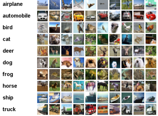
All 10 categories of images in the CIFAR-10 dataset
Here are some random images from the first 5 categories, which the first neural network will ‘see’ and be trained on. The categories are - airplane, automobile, bird, cat, or deer.
Fig: First 5 categories of images, seen only by the first neural network.
But we are actually interested in building a neural net for the last 5 categories of images - dog, frog, horse, sheep, or truck.

Fig: Last 5 categories of images, seen only by the second neural network.
Next, we define two groups/types of layers: feature (convolutions) and classification (dense).
Again, do not be bothered about the implementation details of these code snippets. You can learn the details from any standard tutorial on Keras package. The idea is to understand the concept.
The feature layers:
feature_layers = [
    Conv2D(filters, kernel_size,
           padding='valid',
           input_shape=input_shape),
    Activation('relu'),
    Conv2D(filters, kernel_size),
    Activation('relu'),
    MaxPooling2D(pool_size=pool_size),
    Dropout(0.25),
    Flatten(),
]
The dense classification layer:
classification_layers = [
    Dense(128),
    Activation('relu'),
    Dropout(0.25),
    Dense(num_classes),
    Activation('softmax')
]
Next, we create a complete model by stacking together feature_layers and classification_layers.
model_1 = Sequential(feature_layers + classification_layers)
We then define a function for training the model (not shown) and just train the model for a certain number of epochs to reach a good enough performance:
train_model(model_1,
            (x_train_lt5, y_train_lt5),
            (x_test_lt5, y_test_lt5), num_classes)
We can show how the accuracy of the network evolved over training epochs:
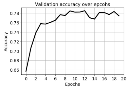
Fig: Validation set accuracy over epochs while training the first network.
Next, we freeze feature layers and rebuild the model.
This freezing of feature layers is at the heart of transfer learning. This allows the re-use of the pre-trained model for classification tasks because users can just stack up to new fully-connected layers on top of the pre-trained feature layers and get good performance.
We will create a fresh new model called model_2 with the untrainable feature_layers and trainable classification_layers. We show the summary in the figure below:
for l in feature_layers:
    l.trainable = False
model_2 = Sequential(feature_layers + classification_layers)
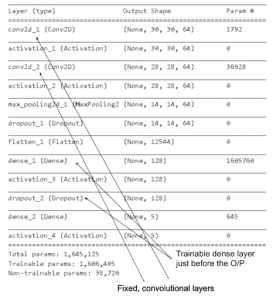
Fig: The model summary of the second network showing the fixed and trainable weights. The fixed weights are transferred directly from the first network.
Now we train the second model and observe how it takes less overall time and still gets equal or higher performance.
train_model(model_2,
(x_train_gte5, y_train_gte5),(x_test_gte5, y_test_gte5), num_classes)
The accuracy of the second model is even higher than the first model, although this may not be the case all the time, and depends on the model architecture and dataset.
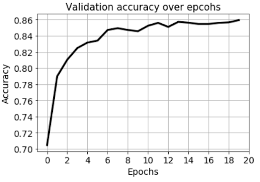
Fig: Validation set accuracy over epochs while training the second network.
The time taken for training two models are shown below:
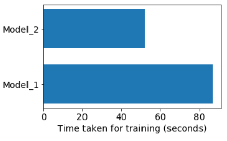
Fig: Training time for the two networks.
What Did We Achieve?
Not only did the model_2 train faster than model_1, it also started at a higher baseline accuracy and achieved better final accuracy for the same number of epochs and identical hyperparameters (learning rate, optimizer, batch size, etc.). And it achieved this training on images that were not seen by model_1.
This means that although model_1 was trained on images of - airplane, automobile, bird, cat, or deer - it’s learned weights, when transferred to model_2, helped model_2 achieve excellent performance on the classification of completely different categories of images - dog, frog, horse, sheep, or truck.
Isn’t that amazing? And you can now build this kind of transfer learning with so few lines of codes. Again, the entire code is open-source and can be found here.


Transfer Learning Made Easy: Coding a Powerful Technique
Artificial Intelligence for the Average User
Artificial intelligence (A.I.) is shaping up to be the most powerful and transformative technology to sweep the globe and touch all facets of life - economics, healthcare, finance, industry, socio-cultural interactions, etc. - in an unprecedented manner. This is even more important with developments in transfer learning and machine learning capabilities.
Already, we are using A.I. technologies on a daily basis, and it is impacting our lives and choices whether we consciously know it or not. From our Google search and Navigation, Netflix movie recommendations, Amazon purchase suggestions, voice assistants for daily tasks like Siri or Alexa, Facebook community building, medical diagnoses, credit score calculations, and mortgage decision making, etc., A.I. is only going to grow in adoption.
Most modern A.I. systems are currently being powered by a family of algorithms or techniques called deep learning, which basically trains and builds deep layers of neural networks with various architectural configurations.
Image source: Fjodor van Veen - asimovinstitute.org
After 50+ years of ebbs and flows, the deep learning revolution has caught the steam and looks unstoppable - fueled by Big Data technologies, innovation in hardware, and algorithms. Therefore, deep learning networks are promising to impact and fundamentally alter how we, humans, live, work, and play for at least the next few decades to come.
So, we can finally see the promise of A.I. for everyone on the planet!
However...there is a catch.

Deep Learning is Expensive and the Focus is Narrow
Deep learning networks tend to be resource-hungry and computationally expensive. Unlike traditional statistical learning models (such as regression, decision trees, or support vector machines), they tend to contain millions of parameters and therefore need a lot of training data to avoid overfitting.
Therefore, deep learning models are trained with massive amounts of high-dimensional raw data such as images, unstructured text, or audio signals. Also, they employ millions of vectorized computation (e.g. matrix multiplication) over and over, to optimize the huge parameter set to fit the data. Moreover, they are built with a large number of hyperparameters (e.g. number of layers, neurons per layer, optimizer algorithm settings, etc.) and it often takes many weeks or months for a team of highly trained researchers to create a state-of-the-art model.
All of these lead to a great demand on the computational power needed to train and robust and high-performance deep learning model, optimized for a given task.
Let’s say we can afford to train a great model after spending a huge amount of computational resources. Don’t we want to re-use this model for the maximum number and variety of tasks and reap the benefit of our investment many times over?
Herein lies the problem.
Deep learning algorithms, so far, have been traditionally designed to work in isolation. These algorithms are trained to solve specific tasks. The models, in most cases, have to be rebuilt from scratch once the feature-space distribution changes.
But, this does not make sense, especially when it is compared to how we humans currently utilize our limited computation speed.
Humans have an inherent ability to transfer knowledge across tasks. What we acquire as knowledge while learning about one task, we utilize in the same way to solve related tasks. If the similarity between the tasks or domains is high, we are able to cross-utilize our ‘learned’ knowledge better.
Transfer learning is the idea of overcoming the isolated learning paradigms and utilizing knowledge acquired for one task to solve related ones, as applied to machine learning, and in particular, to the domain of deep learning.

Image source: A Comprehensive Hands-on Guide to Transfer Learning with Real-World Applications in Deep Learning
Transfer Learning for Deep Learning Networks
There is a myriad of strategies to follow for the transfer learning process in the deep learning setting, and multiple important things to consider and engineering decisions to make - similarity of datasets and domains, supervised or unsupervised setting, how much retraining to be done, etc.
However, to put it very simply, we can assume that for transfer learning:
- We need to take a pre-trained deep learning model
- Re-use all or certain portions of it
- Apply it to our new domain of interest, for a particular machine learning problem–classification or regression.
In this way, we are able to avoid a large portion of the huge computational effort of training and optimizing a large deep learning model.
In the end, a trained deep learning model is just a collection of millions of real numbers in a particular data structure format, which can be used readily for prediction/inference, the task we are really interested in, as the consumers of the model.
But remember that a pre-trained model might have been trained using a particular classification in mind i.e. its output vector and computation graph is suited for the prediction of a particular task only.
Therefore, a widely used strategy in transfer learning is to:
- Load the weights matrices of a pre-trained model except for the weights of the very last layers near the O/P,
- Hold those weights fixed i.e. untrainable
- Attach new layers suitable for the task at hand, and train the model with new data

Fig: The transfer learning strategy for deep learning networks, as we will explore here.
This way, we don’t have to train the whole model, we get to repurpose the model for our specific machine learning task, yet can leverage the learned structures and patterns of the data, contained in the fixed weights, which are loaded from the pre-trained, optimized model.
A Hands-On Example You Can Run on Your Laptop
Let’s get our hands dirty and build a simple code demo to demonstrate the power of transfer learning, shall we?
Why not follow a traditional approach?
Now, traditionally, tutorials on this topic have focused on learning from famous, high-performance deep learning networks, such as VGGNet-16, ResNet-50, or Inception-V3/V4, etc. These networks were trained on the massive ImageNet database, and secured top places in the annual ImageNet competition - ILSVRC, thereby positioning themselves as the golden benchmark models for image classification tasks.
However, the issue with these networks, is that they contain a large number of complex layers, and not easy to understand when you are starting to learn deep learning concepts.
Therefore, if you want to code up a transfer learning example from scratch, it may be beneficial, from self-learning and confidence-building point of view, to try an independent example first. You can train a deep learning model first, transfer its learning to another seed network, and then show the performance on a standard classification task.
What are we going to do in this tutorial?
In this article, we will demonstrate the transfer learning concept in a very simple setting using Python, working with the Keras package (TensorFlow backend). We will take the well-known CIFAR-10 dataset and do the following:
- Create a Keras neural net by stacking a set of classificiation_layers on top of a set of feature_layers
- Train the resulting network on a partial CIFAR-10 dataset, consisting of examples from the first 5 categories (0...4).
- Freeze the feature_layers and stack a new set of fully-connected layers on top of them, thereby creating another conv net
- Train this new conv net on the examples from the rest of the categories (5..9) of CIFAR-10, tuning weights only for those densely connected layers
The entire code is open-source and can be found here. We show only some essential parts of the code here in this article.
Code Along
We start by importing the necessary libraries and functions:
from time import time
import keras
from keras.datasets import mnist,cifar10
from keras.models import Sequential
from keras.layers import Dense, Dropout, Activation, Flatten
from keras.layers import Conv2D, MaxPooling2D
from keras.optimizers import Adam
from keras import backend as K

import matplotlib.pyplot as plt
import random
Next, we decide on some architectural choices for the deep learning models. We will use the convolutional neural net (CNN), as it is the most suited for image classification task:
# number of convolutional filters to use
filters = 64
# size of pooling area for max pooling
pool_size = 2
# convolution kernel size
kernel_size = 3
Next, we split the dataset into training and validation sets, and create two datasets - one with class labels below 5 and one with 5 and above. Why do we do that?
The whole CIFAR-10 dataset has 10 categories of images in a very small size. We will have two neural networks. One will be pre-trained and the learning will be transferred to a second network. But, we will not use all the categories of the image to train both networks. The first one will be trained only using the first 5 categories of images and this learning will help the second network to learn the last 5 categories of images faster.
Therefore,

All 10 categories of images in the CIFAR-10 dataset
Here are some random images from the first 5 categories, which the first neural network will ‘see’ and be trained on. The categories are - airplane, automobile, bird, cat, or deer.
Fig: First 5 categories of images, seen only by the first neural network.
But we are actually interested in building a neural net for the last 5 categories of images - dog, frog, horse, sheep, or truck.

Fig: Last 5 categories of images, seen only by the second neural network.
Next, we define two groups/types of layers: feature (convolutions) and classification (dense).
Again, do not be bothered about the implementation details of these code snippets. You can learn the details from any standard tutorial on Keras package. The idea is to understand the concept.
The feature layers:
feature_layers = [
    Conv2D(filters, kernel_size,
           padding='valid',
           input_shape=input_shape),
    Activation('relu'),
    Conv2D(filters, kernel_size),
    Activation('relu'),
    MaxPooling2D(pool_size=pool_size),
    Dropout(0.25),
    Flatten(),
]
The dense classification layer:
classification_layers = [
    Dense(128),
    Activation('relu'),
    Dropout(0.25),
    Dense(num_classes),
    Activation('softmax')
]
Next, we create a complete model by stacking together feature_layers and classification_layers.
model_1 = Sequential(feature_layers + classification_layers)
We then define a function for training the model (not shown) and just train the model for a certain number of epochs to reach a good enough performance:
train_model(model_1,
            (x_train_lt5, y_train_lt5),
            (x_test_lt5, y_test_lt5), num_classes)
We can show how the accuracy of the network evolved over training epochs:

Fig: Validation set accuracy over epochs while training the first network.
Next, we freeze feature layers and rebuild the model.
This freezing of feature layers is at the heart of transfer learning. This allows the re-use of the pre-trained model for classification tasks because users can just stack up to new fully-connected layers on top of the pre-trained feature layers and get good performance.
We will create a fresh new model called model_2 with the untrainable feature_layers and trainable classification_layers. We show the summary in the figure below:
for l in feature_layers:
    l.trainable = False
model_2 = Sequential(feature_layers + classification_layers)

Fig: The model summary of the second network showing the fixed and trainable weights. The fixed weights are transferred directly from the first network.
Now we train the second model and observe how it takes less overall time and still gets equal or higher performance.
train_model(model_2,
(x_train_gte5, y_train_gte5),(x_test_gte5, y_test_gte5), num_classes)
The accuracy of the second model is even higher than the first model, although this may not be the case all the time, and depends on the model architecture and dataset.

Fig: Validation set accuracy over epochs while training the second network.
The time taken for training two models are shown below:

Fig: Training time for the two networks.
What Did We Achieve?
Not only did the model_2 train faster than model_1, it also started at a higher baseline accuracy and achieved better final accuracy for the same number of epochs and identical hyperparameters (learning rate, optimizer, batch size, etc.). And it achieved this training on images that were not seen by model_1.
This means that although model_1 was trained on images of - airplane, automobile, bird, cat, or deer - it’s learned weights, when transferred to model_2, helped model_2 achieve excellent performance on the classification of completely different categories of images - dog, frog, horse, sheep, or truck.
Isn’t that amazing? And you can now build this kind of transfer learning with so few lines of codes. Again, the entire code is open-source and can be found here.


