Deep Learning
Automated Machine Learning with AutoKeras - Image, Text, & Structured Data
January 26, 2024
13 min read


AutoML is the process of automating the whole process of applying machine learning to real world problems. With aims to automate architecture and hyperparameter search and return an optimal model for a given dataset, AutoML potentially includes all stages of deploying a machine learning algorithm from start to finish.
In this article, we’ll introduce ourselves to one prominent AutoML library via Keras. We’ll deep dive into the understandings needed to facilitate AutoML, and go through a few examples of AutoML with AutoKeras to solve problems in some of the most common application areas, images classificiation, text classification, and structured data analysis. It starts with this code block:
import autokeras as ak
import sklearn.datasets
my_x, my_y= sklearn.datasets.load_digits(return_X_y=True)
x_train, y_train = my_x[0:1200].reshape(-1,8,8), my_y[0:1200]
x_test, y_test = my_x[1200:1400].reshape(-1,8,8), my_y[1200:1400]

classifier = autokeras.ImageClassifier()
history = classifier.fit(x_train, y_train)

results = classifier.predict(x_test)
That seems… too easy? Ideally, AutoML can not only automate solutions for common types of problems, but also offer better results efficiently compared to manually choosing hyperparameters in a guess and check fashion. Afterall, machine learning and optimization is a math problem, and computers, algorithms, and AI training is all about math.
You can find code for all the examples in this post hosted as a Kaggle notebook.
Image classification started us off modern machine learning when AlexNet gave us a glimpse into the promise of scale in image recognition. And now, image recognition is a basic machine learning task to train and deploy for many machine learning enthusiasts. How does AutoML apply to image classification problem? First, let’s break down all 8 lines in the code snippet from earlier and have a look at each piece.
We have a few lightweight imports: SciKit-Learn, the AutoKeras library itself, and NumPy, and matplotlib. The sklearn.datasets module we’ll use for training data a Python modules that has to be imported explicitly – importing sklearn and calling sklearn.datasets is invalid. In fact, you don’t even need to import the parent library either.
import autokeras as ak
import sklearn.datasets
import matplotlib.pyplot as plt
plt.xkcd()
import numpy as np
We use sklearn.datasets in these examples just to provide easy access to demo datasets. For image classification, we use digits, which a small take on the hand-written digit recognition program. These are provided as N by 64 pixels in a NumPy array, so they’ll need to be reshaped to have height and width of 8 to be viewable as images.
Here we manual chose training/validation/test split of 1200/397/200. AutoKeras model for image classification uses its a default validation split of 0.8/0.2, so manually providing a validation split is not required. However, relying on the fit method to handle the split according to validation_split (whether provided explicitly or using the default value of 0.2), the returning history object only includes training loss and accuracy. Therefore, the full example below uses a manual validation split so we can see other important training info.
my_x, my_y= sklearn.datasets.load_digits(return_X_y=True)

x_train, y_train = my_x[0:1200].reshape(-1,8,8), my_y[0:1200]
x_test, y_test = my_x[1200:1400].reshape(-1,8,8), my_y[1200:1400]
x_val, y_val = my_x[1400:].reshape(-1,8,8), my_y[1400:]
You can rely on the defaults when instantiating the ImageClassifier class from AutoKeras, or fine tune by providing constraints. Many of the class instantiation arguments, such as the number of classes and whether to use binary cross entropy or cross entropy loss can be inferred from the training data when the fit method is called.
One argument parameter you probably should define explicitly is the random seed to ensure results are not by chance AND so that someone can re-run your experiments and get the same results. A random seed is a randomly defined set of training data and validation data where a defined seed ensure training and validation data is divided the same every time. Random seeds are not hyperparameters!
You can also define the maximum number of different trials for the AutoML algorithm to try. More trials mean more chances to get it right, but at the expense of more compute time. For our small demo problem, we probably won’t need the default 100 max_trials to maximize accuracy.
classifier = autokeras.ImageClassifier(seed=42, \
            max_trials=32, tuner="bayesian")
The fit method returns a Keras history, the training record for the best model. This is also where you can specify a certain number of epochs to train for during each trial. The default is 100, and we probably also don’t for this small of a dataset.
history = classifier.fit(x_train, y_train, \
validation_data=(x_val, y_val), max_trials=32)
During training, AutoKeras will print some information about the trials and what parameters are being used and varied throughout the process. These include dropout, the optimizer being used, info about the model architecture being used, etc.
Search: Running Trial #1

Value             |Best Value So Far |Hyperparameter
True              |True              |image_block_1/normalize
False             |False             |image_block_1/augment
xception          |xception          |image_block_1/block_type
flatten           |flatten           |classification_head_1/spatial_reduction_1/reduction_type
0.5               |0.5               |classification_head_1/dropout
sgd               |sgd               |optimizer
0.0001            |0.0001            |learning_rate
You can get a feel for how the training went (for the best model) by plotting the history and checking performance on the test set.
fig, ax = plt.subplots(2,1)
ax2 = ax[1]
ax = ax[0]
ax.plot(history.history["loss"], "g", lw=3, label="training loss")
ax2.plot(history.history["accuracy"],"b", lw=3, label="training accuracy")
ax.plot(history.history["val_loss"],"k", lw=3, label="validation loss")
ax2.plot(history.history["val_accuracy"], "r", lw=3, label="validation accuracy")
ax.set_title("Image Classification Demo with AutoKeras")
ax.legend()
ax2.legend()
plt.savefig("image_demo.png")
plt.show()
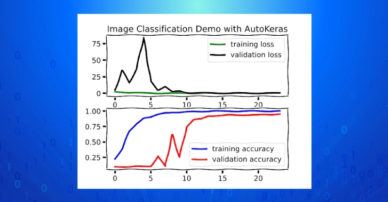
We can also assess the best model in terms of test set accuracy using NumPy.
results = np.array(classifier.predict(x_test), dtype=int)
accuracy = np.mean(results.squeeze() ==  y_test[0:3])
print(f"Image classification test accuracy = {accuracy:4f}")

>>Image classification test accuracy = 0.995000
For our structured data demo, we’ll use the StructuredDataRegressor class from AutoKeras to solve another demo problem using diabetes dataset from sklearn. The objective of this dataset is to predict a numerical measure of disease progression using a set of 10 features including age, sex, BMI, blood pressure, and a number of measurements of relevant blood serum constituents.
The dataset is small with only 442 samples; try this AutoML demo on a larger dataset and use the California housing price prediction dataset, which has 20,640 samples.
my_x, my_y = sklearn.datasets.load_diabetes(return_X_y=True)
#sklearn.datasets.fetch_california_housing(return_X_y=True)

split = int(0.1*my_x.shape[0])

def normalize_y(my_y):
# normalize my_y to have mean 0 and std. dev. 1.0

mean_y = np.mean(my_y)
std_dev_y = np.std(my_y)

return (my_y - mean_y) / std_dev_y, mean_y, std_dev_y

def denormalize_y(my_y, my_mean, my_std_dev):
# return predicted values to y to the original range

return my_y * my_std_dev +  my_mean

my_y, my_mean, my_std_dev = normalize_y(my_y)

split = int(0.1*my_x.shape[0])

x_train, y_train = my_x[:-2*split], my_y[:-2*split]
x_test, y_test = my_x[-2*split:-split], my_y[-2*split:-split]
x_val, y_val = my_x[-split:], my_y[-split:]
The StructuredDataRegressor model is instantiated as before, and we will again call the fit method with an explicit validation_data dataset.
regression_model = autokeras.StructuredDataRegressor(\
        seed=42, max_trials=16)
history = regression_model.fit(x_train, y_train, \
        validation_data=(x_val, y_val), epochs=32)

plt.figure()
plt.plot(history.history["loss"], \
lw=3, label="training MSE")
plt.plot(history.history["val_loss"], \
lw=3, label="validation MSE")
plt.title("Structured Data Regression Demo with AutoKeras")
plt.legend()
plt.show()
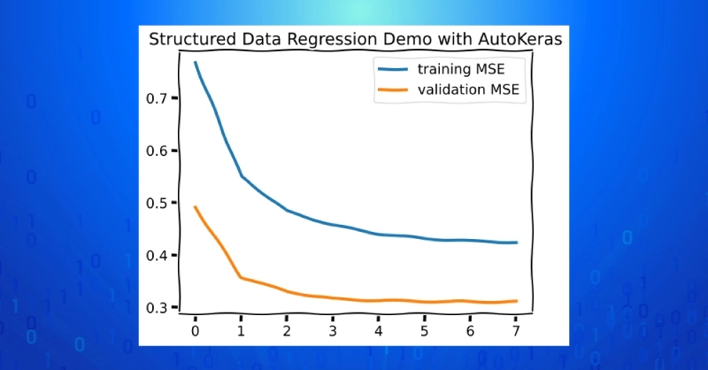
mse_loss = lambda x1, x2: np.mean((x1-x2)**2)

results = regression_model.predict(x_test)

my_mse = mse_loss(y_test, results)
print(f"Test MSE = {my_mse:4f}")

>> Test MSE = 1.764508
For text classification we’ll use the 20newsgroups dataset from sklearn. The full version of this dataset has 20 classes and 11,314 samples, but we’ll cut that down to 2,373 samples by only considering the samples with a science topic label. The train/validation/test split is manually implemented as before. To run the demo on all 20 classes, omit the categories argument or set it to None.
#classes = None
classes= ["sci.crypt", "sci.electronics", "sci.med", "sci.space"]
text_twenty = sklearn.datasets.fetch_20newsgroups(categories=classes)

split = int(0.1 * len(text_twenty["data"]))

x_train = text_twenty["data"][:-2*split]
y_train = text_twenty["target"][:-2*split]

x_val = text_twenty["data"][-split:]
y_val = text_twenty["target"][-split:]

x_test = text_twenty["data"][-2*split:-split]
y_test = text_twenty["target"][-2*split:-split]
Unlike the previous examples we don’t pass the validation split to the fit method due to a bug in the callback that gets called at the end of training (see caveat section). Instead, we’ll take advantage of the validation_split argument (though this can be left at the default value of 0.2).
text_classifier = autokeras.TextClassifier(max_trials=8, \
        seed=42, tuner="random")
history = text_classifier.fit(np.array(x_train), y_train, \
     validation_data=(np.array(x_val), y_val), epochs=my_epochs)

fig, ax = plt.subplots(1,1)
ax2 = ax.twinx()
ax.plot(history.history["loss"], lw=3, label="training loss")
ax2.plot(history.history["accuracy"], lw=3, label="training accuracy")

ax.plot(history.history["val_loss"], lw=3, label="validation loss")
ax2.plot(history.history["val_accuracy"], lw=3, label="validation accuracy")
plt.title("Text Classification Demo with AutoKeras")
plt.legend()
plt.savefig("text_demo.png")
plt.show()
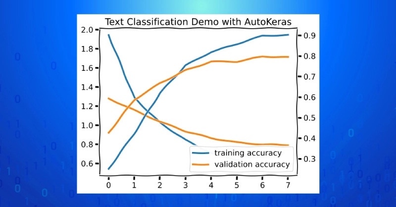
We can plot the best training run and calculate test accuracy explicitly to gauge the final performance of the best model.
predict_test = text_classifier.predict(np.array(x_val))
predict_test = np.array(predict_test.squeeze(), dtype=int)

test_accuracy = np.mean(predict_test ==  y_test)

print(f"test set accuracy: {test_accuracy:4f}")

# A large validation-test performance gap indicates overfitting to the validation set. That’s why holding out the test set is important!
>>validation accuracy: 0.793249
>>test set accuracy: 0.270042
While AutoKeras is a useful library for automated ML, it’s not magic and does have some bugs and drawbacks. Still AutoML address these problems if willing to pay the cost.
As mentioned in memory usage, there is one significant bug with the max_model_size argument. That being said, this is an open-source project under active development (under an Apache 2.0 license), which means that anyone that finds problems is encouraged to submit issues and fixes themselves. They have a contribution guide and plenty of work is available to contribute, so rough edges should not be a dealbreaker for using the library.
Given a new problem, should a data scientist/machine learning practitioner roll their own approach based on intuition, experience, and a recipe book of past projects, or should one use AutoML? The answer is, as with so many things, it depends.
If you have a problem for which you already have an effective training recipe, you should probably use it and avoid the additional time and computational required to explore variations in the space of all possible training runs for that data type. However, if you encounter a novel problem and want to get a gauge on what an AutoML may adjust according to hyperparameters, there are potential efficiency improvements in the systematic approach of AutoML.
AutoML is a good way to explore and experiment solutions in a systematized way (and avoid the inherent inefficiencies of manually searching and tuning). AutoML also may provide a way to circumvent problems with a novel problem that can even teach us different parameter optimizations. In all cases, AutoML should be considered as another tool to help data scientists achieve better results and should never be used without caution, tweaking, or complete rebuild, and many machine learning practitioners that use AutoML treat is a such.
AutoML is great for proof of concepts in developing robust machine learning and AI models. Train your own robust models with an Exxact Workstations equipped with the latest GPU hardware. Contact us today for more information on availability and discounts.
AutoML is the process of automating the whole process of applying machine learning to real world problems. With aims to automate architecture and hyperparameter search and return an optimal model for a given dataset, AutoML potentially includes all stages of deploying a machine learning algorithm from start to finish.
In this article, we’ll introduce ourselves to one prominent AutoML library via Keras. We’ll deep dive into the understandings needed to facilitate AutoML, and go through a few examples of AutoML with AutoKeras to solve problems in some of the most common application areas, images classificiation, text classification, and structured data analysis. It starts with this code block:
import autokeras as ak
import sklearn.datasets
my_x, my_y= sklearn.datasets.load_digits(return_X_y=True)
x_train, y_train = my_x[0:1200].reshape(-1,8,8), my_y[0:1200]
x_test, y_test = my_x[1200:1400].reshape(-1,8,8), my_y[1200:1400]

classifier = autokeras.ImageClassifier()
history = classifier.fit(x_train, y_train)

results = classifier.predict(x_test)
That seems… too easy? Ideally, AutoML can not only automate solutions for common types of problems, but also offer better results efficiently compared to manually choosing hyperparameters in a guess and check fashion. Afterall, machine learning and optimization is a math problem, and computers, algorithms, and AI training is all about math.
You can find code for all the examples in this post hosted as a Kaggle notebook.
Image classification started us off modern machine learning when AlexNet gave us a glimpse into the promise of scale in image recognition. And now, image recognition is a basic machine learning task to train and deploy for many machine learning enthusiasts. How does AutoML apply to image classification problem? First, let’s break down all 8 lines in the code snippet from earlier and have a look at each piece.
We have a few lightweight imports: SciKit-Learn, the AutoKeras library itself, and NumPy, and matplotlib. The sklearn.datasets module we’ll use for training data a Python modules that has to be imported explicitly – importing sklearn and calling sklearn.datasets is invalid. In fact, you don’t even need to import the parent library either.
import autokeras as ak
import sklearn.datasets
import matplotlib.pyplot as plt
plt.xkcd()
import numpy as np
We use sklearn.datasets in these examples just to provide easy access to demo datasets. For image classification, we use digits, which a small take on the hand-written digit recognition program. These are provided as N by 64 pixels in a NumPy array, so they’ll need to be reshaped to have height and width of 8 to be viewable as images.
Here we manual chose training/validation/test split of 1200/397/200. AutoKeras model for image classification uses its a default validation split of 0.8/0.2, so manually providing a validation split is not required. However, relying on the fit method to handle the split according to validation_split (whether provided explicitly or using the default value of 0.2), the returning history object only includes training loss and accuracy. Therefore, the full example below uses a manual validation split so we can see other important training info.
my_x, my_y= sklearn.datasets.load_digits(return_X_y=True)

x_train, y_train = my_x[0:1200].reshape(-1,8,8), my_y[0:1200]
x_test, y_test = my_x[1200:1400].reshape(-1,8,8), my_y[1200:1400]
x_val, y_val = my_x[1400:].reshape(-1,8,8), my_y[1400:]
You can rely on the defaults when instantiating the ImageClassifier class from AutoKeras, or fine tune by providing constraints. Many of the class instantiation arguments, such as the number of classes and whether to use binary cross entropy or cross entropy loss can be inferred from the training data when the fit method is called.
One argument parameter you probably should define explicitly is the random seed to ensure results are not by chance AND so that someone can re-run your experiments and get the same results. A random seed is a randomly defined set of training data and validation data where a defined seed ensure training and validation data is divided the same every time. Random seeds are not hyperparameters!
You can also define the maximum number of different trials for the AutoML algorithm to try. More trials mean more chances to get it right, but at the expense of more compute time. For our small demo problem, we probably won’t need the default 100 max_trials to maximize accuracy.
classifier = autokeras.ImageClassifier(seed=42, \
            max_trials=32, tuner="bayesian")
The fit method returns a Keras history, the training record for the best model. This is also where you can specify a certain number of epochs to train for during each trial. The default is 100, and we probably also don’t for this small of a dataset.
history = classifier.fit(x_train, y_train, \
validation_data=(x_val, y_val), max_trials=32)
During training, AutoKeras will print some information about the trials and what parameters are being used and varied throughout the process. These include dropout, the optimizer being used, info about the model architecture being used, etc.
Search: Running Trial #1

Value             |Best Value So Far |Hyperparameter
True              |True              |image_block_1/normalize
False             |False             |image_block_1/augment
xception          |xception          |image_block_1/block_type
flatten           |flatten           |classification_head_1/spatial_reduction_1/reduction_type
0.5               |0.5               |classification_head_1/dropout
sgd               |sgd               |optimizer
0.0001            |0.0001            |learning_rate
You can get a feel for how the training went (for the best model) by plotting the history and checking performance on the test set.
fig, ax = plt.subplots(2,1)
ax2 = ax[1]
ax = ax[0]
ax.plot(history.history["loss"], "g", lw=3, label="training loss")
ax2.plot(history.history["accuracy"],"b", lw=3, label="training accuracy")
ax.plot(history.history["val_loss"],"k", lw=3, label="validation loss")
ax2.plot(history.history["val_accuracy"], "r", lw=3, label="validation accuracy")
ax.set_title("Image Classification Demo with AutoKeras")
ax.legend()
ax2.legend()
plt.savefig("image_demo.png")
plt.show()
We can also assess the best model in terms of test set accuracy using NumPy.
results = np.array(classifier.predict(x_test), dtype=int)
accuracy = np.mean(results.squeeze() ==  y_test[0:3])
print(f"Image classification test accuracy = {accuracy:4f}")

>>Image classification test accuracy = 0.995000
For our structured data demo, we’ll use the StructuredDataRegressor class from AutoKeras to solve another demo problem using diabetes dataset from sklearn. The objective of this dataset is to predict a numerical measure of disease progression using a set of 10 features including age, sex, BMI, blood pressure, and a number of measurements of relevant blood serum constituents.
The dataset is small with only 442 samples; try this AutoML demo on a larger dataset and use the California housing price prediction dataset, which has 20,640 samples.
my_x, my_y = sklearn.datasets.load_diabetes(return_X_y=True)
#sklearn.datasets.fetch_california_housing(return_X_y=True)

split = int(0.1*my_x.shape[0])

def normalize_y(my_y):
# normalize my_y to have mean 0 and std. dev. 1.0

mean_y = np.mean(my_y)
std_dev_y = np.std(my_y)

return (my_y - mean_y) / std_dev_y, mean_y, std_dev_y

def denormalize_y(my_y, my_mean, my_std_dev):
# return predicted values to y to the original range

return my_y * my_std_dev +  my_mean

my_y, my_mean, my_std_dev = normalize_y(my_y)

split = int(0.1*my_x.shape[0])

x_train, y_train = my_x[:-2*split], my_y[:-2*split]
x_test, y_test = my_x[-2*split:-split], my_y[-2*split:-split]
x_val, y_val = my_x[-split:], my_y[-split:]
The StructuredDataRegressor model is instantiated as before, and we will again call the fit method with an explicit validation_data dataset.
regression_model = autokeras.StructuredDataRegressor(\
        seed=42, max_trials=16)
history = regression_model.fit(x_train, y_train, \
        validation_data=(x_val, y_val), epochs=32)

plt.figure()
plt.plot(history.history["loss"], \
lw=3, label="training MSE")
plt.plot(history.history["val_loss"], \
lw=3, label="validation MSE")
plt.title("Structured Data Regression Demo with AutoKeras")
plt.legend()
plt.show()
mse_loss = lambda x1, x2: np.mean((x1-x2)**2)

results = regression_model.predict(x_test)

my_mse = mse_loss(y_test, results)
print(f"Test MSE = {my_mse:4f}")

>> Test MSE = 1.764508
For text classification we’ll use the 20newsgroups dataset from sklearn. The full version of this dataset has 20 classes and 11,314 samples, but we’ll cut that down to 2,373 samples by only considering the samples with a science topic label. The train/validation/test split is manually implemented as before. To run the demo on all 20 classes, omit the categories argument or set it to None.
#classes = None
classes= ["sci.crypt", "sci.electronics", "sci.med", "sci.space"]
text_twenty = sklearn.datasets.fetch_20newsgroups(categories=classes)

split = int(0.1 * len(text_twenty["data"]))

x_train = text_twenty["data"][:-2*split]
y_train = text_twenty["target"][:-2*split]

x_val = text_twenty["data"][-split:]
y_val = text_twenty["target"][-split:]

x_test = text_twenty["data"][-2*split:-split]
y_test = text_twenty["target"][-2*split:-split]
Unlike the previous examples we don’t pass the validation split to the fit method due to a bug in the callback that gets called at the end of training (see caveat section). Instead, we’ll take advantage of the validation_split argument (though this can be left at the default value of 0.2).
text_classifier = autokeras.TextClassifier(max_trials=8, \
        seed=42, tuner="random")
history = text_classifier.fit(np.array(x_train), y_train, \
     validation_data=(np.array(x_val), y_val), epochs=my_epochs)

fig, ax = plt.subplots(1,1)
ax2 = ax.twinx()
ax.plot(history.history["loss"], lw=3, label="training loss")
ax2.plot(history.history["accuracy"], lw=3, label="training accuracy")

ax.plot(history.history["val_loss"], lw=3, label="validation loss")
ax2.plot(history.history["val_accuracy"], lw=3, label="validation accuracy")
plt.title("Text Classification Demo with AutoKeras")
plt.legend()
plt.savefig("text_demo.png")
plt.show()
We can plot the best training run and calculate test accuracy explicitly to gauge the final performance of the best model.
predict_test = text_classifier.predict(np.array(x_val))
predict_test = np.array(predict_test.squeeze(), dtype=int)

test_accuracy = np.mean(predict_test ==  y_test)

print(f"test set accuracy: {test_accuracy:4f}")

# A large validation-test performance gap indicates overfitting to the validation set. That’s why holding out the test set is important!
>>validation accuracy: 0.793249
>>test set accuracy: 0.270042
While AutoKeras is a useful library for automated ML, it’s not magic and does have some bugs and drawbacks. Still AutoML address these problems if willing to pay the cost.
As mentioned in memory usage, there is one significant bug with the max_model_size argument. That being said, this is an open-source project under active development (under an Apache 2.0 license), which means that anyone that finds problems is encouraged to submit issues and fixes themselves. They have a contribution guide and plenty of work is available to contribute, so rough edges should not be a dealbreaker for using the library.
Given a new problem, should a data scientist/machine learning practitioner roll their own approach based on intuition, experience, and a recipe book of past projects, or should one use AutoML? The answer is, as with so many things, it depends.
If you have a problem for which you already have an effective training recipe, you should probably use it and avoid the additional time and computational required to explore variations in the space of all possible training runs for that data type. However, if you encounter a novel problem and want to get a gauge on what an AutoML may adjust according to hyperparameters, there are potential efficiency improvements in the systematic approach of AutoML.
AutoML is a good way to explore and experiment solutions in a systematized way (and avoid the inherent inefficiencies of manually searching and tuning). AutoML also may provide a way to circumvent problems with a novel problem that can even teach us different parameter optimizations. In all cases, AutoML should be considered as another tool to help data scientists achieve better results and should never be used without caution, tweaking, or complete rebuild, and many machine learning practitioners that use AutoML treat is a such.
AutoML is great for proof of concepts in developing robust machine learning and AI models. Train your own robust models with an Exxact Workstations equipped with the latest GPU hardware. Contact us today for more information on availability and discounts.