Deep Learning
Diffusion and Denoising - Explaining Text-to-Image Generative AI
March 29, 2024
15 min read

Denoising diffusion models are trained to pull patterns out of noise, to generate a desirable image. The training process involves showing model examples of images (or other data) with varying levels of noise determined according to a noise scheduling algorithm, intending to predict what parts of the data are noise. If successful, the noise prediction model will be able to gradually build up a realistic-looking image from pure noise, subtracting increments of noise from the image at each time step.
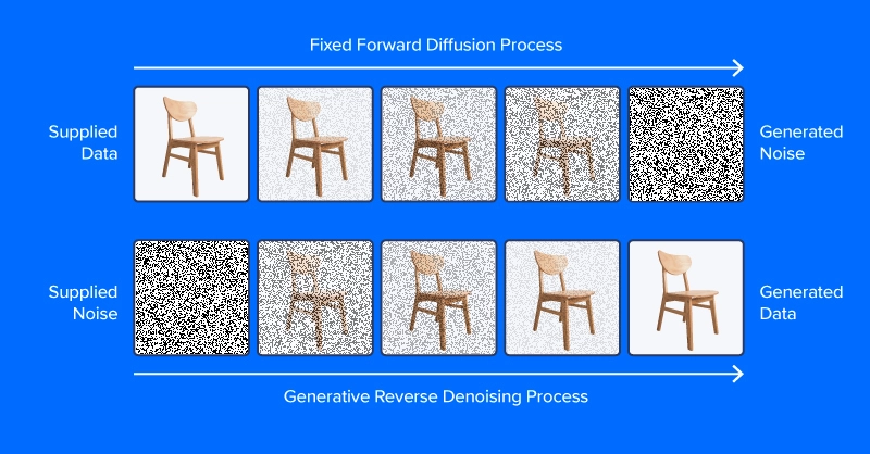
Unlike the image at the top of this section, modern diffusion models don’t predict noise from an image with added noise, at least not directly. Instead, they predict noise in a latent space representation of the image. Latent space represents images in a compressed set of numerical features, the output of an encoding module from a variational autoencoder, or VAE. This trick put the “latent” in latent diffusion, and greatly reduced the time and computational requirements for generating images. As reported by the paper authors, latent diffusion speeds up inference by at least ~2.7X over direct diffusion and trains about three times faster.
People working with latent diffusion often talk of using a “diffusion model,” but in fact, the diffusion process employs several modules. As in the diagram above, a diffusion pipeline for text-to-image workflows typically includes a text embedding model (and its tokenizer), a denoise prediction/diffusion model, and an image decoder. Another important part of latent diffusion is the scheduler, which determines how the noise is scaled and updated over a series of “time steps” (a series of iterative updates that gradually remove noise from latent space).
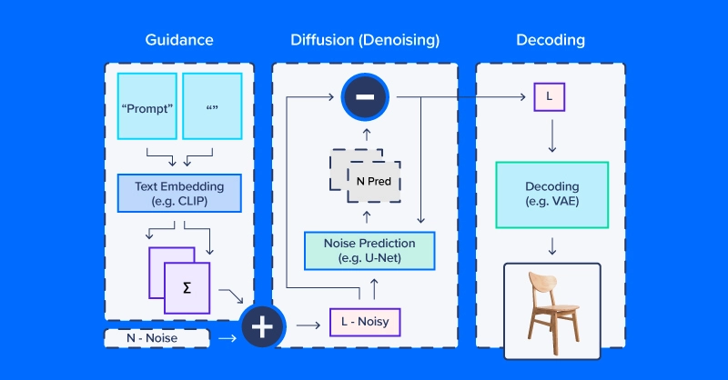
We’ll use CompVis/latent-diffusion-v1-4 for most of our examples. Text embedding is handled by a CLIPTextModel and CLIPTokenizer. Noise prediction uses a ‘U-Net,’ a type of image-to-image model that originally gained traction as a model for applications in biomedical images (especially segmentation). To generate images from denoised latent arrays, the pipeline uses a variational autoencoder (VAE) for image decoding, turning those arrays into images.
We’ll start by building our version of this pipeline from HuggingFace components.
# local setup
virtualenv diff_env –python=python3.8
source diff_env/bin/activate
pip install diffusers transformers huggingface-hub
pip install torch --index-url https://download.pytorch.org/whl/cu118
Make sure to check pytorch.org to ensure the right version for your system if you’re working locally. Our imports are relatively straightforward, and the code snippet below suffices for all the following demos.
import os
import numpy as np
import torch
from diffusers import StableDiffusionPipeline, AutoPipelineForImage2Image
from diffusers.pipelines.pipeline_utils import numpy_to_pil
from transformers import CLIPTokenizer, CLIPTextModel
from diffusers import AutoencoderKL, UNet2DConditionModel, \
       PNDMScheduler, LMSDiscreteScheduler

from PIL import Image
import matplotlib.pyplot as plt
Now for the details. Start by defining image and diffusion parameters and a prompt.
prompt = [" "]

# image settings
height, width = 512, 512

# diffusion settings
number_inference_steps = 64
guidance_scale = 9.0
batch_size = 1
Initialize your pseudorandom number generator with a seed of your choice for reproducing your results.
def seed_all(seed):
    torch.manual_seed(seed)
    np.random.seed(seed)

seed_all(193)
Now we can initialize the text embedding model, autoencoder, a U-Net, and the time step scheduler.
tokenizer = CLIPTokenizer.from_pretrained("openai/clip-vit-large-patch14")
text_encoder = CLIPTextModel.from_pretrained("openai/clip-vit-large-patch14")
vae = AutoencoderKL.from_pretrained("CompVis/stable-diffusion-v1-4", \
        subfolder="vae")
unet = UNet2DConditionModel.from_pretrained("CompVis/stable-diffusion-v1-4",\
        subfolder="unet")
scheduler = PNDMScheduler()
scheduler.set_timesteps(number_inference_steps)

my_device = torch.device("cuda") if torch.cuda.is_available() else torch.device("cpu")
vae = vae.to(my_device)
text_encoder = text_encoder.to(my_device)
unet = unet.to(my_device)
Encoding the text prompt as an embedding requires first tokenizing the string input. Tokenization replaces characters with integer codes corresponding to a vocabulary of semantic units, e.g. via byte pair encoding (BPE). Our pipeline embeds a null prompt (no text) alongside the textual prompt for our image. This balances the diffusion process between the provided description and natural-appearing images in general. We’ll see how to change the relative weighting of these components later in this article.
prompt = prompt * batch_size
tokens = tokenizer(prompt, padding="max_length",\
max_length=tokenizer.model_max_length, truncation=True,\
        return_tensors="pt")

empty_tokens = tokenizer([""] * batch_size, padding="max_length",\
max_length=tokenizer.model_max_length, truncation=True,\
        return_tensors="pt")


with torch.no_grad():
    text_embeddings = text_encoder(tokens.input_ids.to(my_device))[0]
    max_length = tokens.input_ids.shape[-1]
    notext_embeddings = text_encoder(empty_tokens.input_ids.to(my_device))[0]
    text_embeddings = torch.cat([notext_embeddings, text_embeddings])
We initialize latent space as random normal noise and scale it according to our diffusion time step scheduler.
latents = torch.randn(batch_size, unet.config.in_channels, \
        height//8, width//8)
latents = (latents * scheduler.init_noise_sigma).to(my_device)
Everything is ready to go, and we can dive into the diffusion loop itself. We can keep track of images by sampling periodically throughout so we can see how noise is gradually decreased.
images = []
display_every = number_inference_steps // 8

# diffusion loop
for step_idx, timestep in enumerate(scheduler.timesteps):
    with torch.no_grad():
        # concatenate latents, to run null/text prompt in parallel.
        model_in = torch.cat([latents] * 2)
        model_in = scheduler.scale_model_input(model_in,\
                timestep).to(my_device)
        predicted_noise = unet(model_in, timestep, \
                encoder_hidden_states=text_embeddings).sample
        # pnu - empty prompt unconditioned noise prediction
        # pnc - text prompt conditioned noise prediction
        pnu, pnc = predicted_noise.chunk(2)
        # weight noise predictions according to guidance scale
        predicted_noise = pnu + guidance_scale * (pnc - pnu)
        # update the latents
        latents = scheduler.step(predicted_noise, \
                timestep, latents).prev_sample
        # Periodically log images and print progress during diffusion
        if step_idx % display_every == 0\
                or step_idx + 1 == len(scheduler.timesteps):
           image = vae.decode(latents / 0.18215).sample[0]
           image = ((image / 2.) + 0.5).cpu().permute(1,2,0).numpy()
           image = np.clip(image, 0, 1.0)
           images.extend(numpy_to_pil(image))
           print(f"step {step_idx}/{number_inference_steps}: {timestep:.4f}")
At the end of the diffusion process, we have a decent rendering of what you wanted to generate. Next, we’ll go over additional techniques for greater control. As we’ve already made our diffusion pipeline, we can use the streamlined diffusion pipeline from HuggingFace for the rest of our examples.
With the latest CPUs and most powerful GPUs available, accelerate your deep learning and AI project optimized to your deployment, budget, and desired performance!
Configure NowWe’ll use a set of helper functions in this section:
def seed_all(seed):
    torch.manual_seed(seed)
    np.random.seed(seed)

def grid_show(images, rows=3):
    number_images = len(images)
    height, width = images[0].size
    columns = int(np.ceil(number_images / rows))
    grid = np.zeros((height*rows,width*columns,3))
    for ii, image in enumerate(images):
        grid[ii//columns*height:ii//columns*height+height, \
                ii%columns*width:ii%columns*width+width] = image
        fig, ax = plt.subplots(1,1, figsize=(3*columns, 3*rows))
        ax.imshow(grid / grid.max())
    return grid, fig, ax

def callback_stash_latents(ii, tt, latents):
    # adapted from fastai/diffusion-nbs/stable_diffusion.ipynb
    latents = 1.0 / 0.18215 * latents
    image = pipe.vae.decode(latents).sample[0]
    image = (image / 2. + 0.5).cpu().permute(1,2,0).numpy()
    image = np.clip(image, 0, 1.0)
    images.extend(pipe.numpy_to_pil(image))

my_seed = 193
We’ll start with the most well-known and straightforward application of diffusion models: image generation from textual prompts, known as text-to-image generation. The model we’ll use was released into the wild (of the Hugging Face Hub) by the academic lab that published the latent diffusion paper. Hugging Face coordinates workflows like latent diffusion via the convenient pipeline API. We want to define what device and what floating point to calculate based on if we have or do not have a GPU.
if (1):
    #Run CompVis/stable-diffusion-v1-4 on GPU
    pipe_name = "CompVis/stable-diffusion-v1-4"
    my_dtype = torch.float16
    my_device = torch.device("cuda")
    my_variant = "fp16"
    pipe = StableDiffusionPipeline.from_pretrained(pipe_name,\
    safety_checker=None, variant=my_variant,\
        torch_dtype=my_dtype).to(my_device)
else:
    #Run CompVis/stable-diffusion-v1-4 on CPU
    pipe_name = "CompVis/stable-diffusion-v1-4"
    my_dtype = torch.float32
    my_device = torch.device("cpu")
    pipe = StableDiffusionPipeline.from_pretrained(pipe_name, \
            torch_dtype=my_dtype).to(my_device)
If you use a very unusual text prompt (very unlike those in the dataset), it’s possible to end up in a less-traveled part of latent space. The null prompt embedding provides a balance and combining the two according to guidance_scale allows you to trade off the specificity of your prompt against common image characteristics.
guidance_images = []
for guidance in [0.25, 0.5, 1.0, 2.0, 4.0, 6.0, 8.0, 10.0, 20.0]:
    seed_all(my_seed)
    my_output = pipe(my_prompt, num_inference_steps=50, \
    num_images_per_prompt=1, guidance_scale=guidance)
    guidance_images.append(my_output.images[0])
    for ii, img in enumerate(my_output.images):
        img.save(f"prompt_{my_seed}_g{int(guidance*2)}_{ii}.jpg")

temp = grid_show(guidance_images, rows=3)
plt.savefig("prompt_guidance.jpg")
plt.show()
Since we generated the prompt using the 9 guidance coefficients, you can plot the prompt and view how the diffusion developed. The default guidance coefficient is 0.75 so on the 7th image would be the default image output.
Sometimes latent diffusion really “wants” to produce an image that doesn’t match your intentions. In these scenarios, you can use a negative prompt to push the diffusion process away from undesirable outputs. For example, we could use a negative prompt to make our Martian astronaut diffusion outputs a little less human.
my_prompt = " "
my_negative_prompt = " "

output_x = pipe(my_prompt, num_inference_steps=50, num_images_per_prompt=9, \
        negative_prompt=my_negative_prompt)

temp = grid_show(output_x)
plt.show()
You should receive outputs that follow your prompt while avoiding outputting the things described in your negative prompt.
Text-to-image generation from scratch is not the only application for diffusion pipelines. Actually, diffusion is well-suited for image modification, starting from an initial image. We’ll use a slightly different pipeline and pre-trained model tuned for image-to-image diffusion.
pipe_img2img = AutoPipelineForImage2Image.from_pretrained(\

        "runwayml/stable-diffusion-v1-5", safety_checker=None,\

torch_dtype=my_dtype, use_safetensors=True).to(my_device)
One application of this approach is to generate variations on a theme. A concept artist might use this technique to quickly iterate different ideas for illustrating an exoplanet based on the latest research.
We’ll first download a public domain artist’s concept of planet 1e in the TRAPPIST system (credit: NASA/JPL-Caltech). Then, after downscaling to remove details, we’ll use a diffusion pipeline to make several different versions of the exoplanet TRAPPIST-1e.
url = \
"https://upload.wikimedia.org/wikipedia/commons/thumb/3/38/TRAPPIST-1e_artist_impression_2018.png/600px-TRAPPIST-1e_artist_impression_2018.png"
img_path = url.split("/")[-1]
if not (os.path.exists("600px-TRAPPIST-1e_artist_impression_2018.png")):
    os.system(f"wget \     '{url}'")
    init_image = Image.open(img_path)

seed_all(my_seed)

trappist_prompt = "Artist's impression of TRAPPIST-1e"\
                  "large Earth-like water-world exoplanet with oceans,"\
                  "NASA, artist concept, realistic, detailed, intricate"

my_negative_prompt = "cartoon, sketch, orbiting moon"

my_output_trappist1e = pipe_img2img(prompt=trappist_prompt, num_images_per_prompt=9, \
     image=init_image, negative_prompt=my_negative_prompt, guidance_scale=6.0)

grid_show(my_output_trappist1e.images)
plt.show()
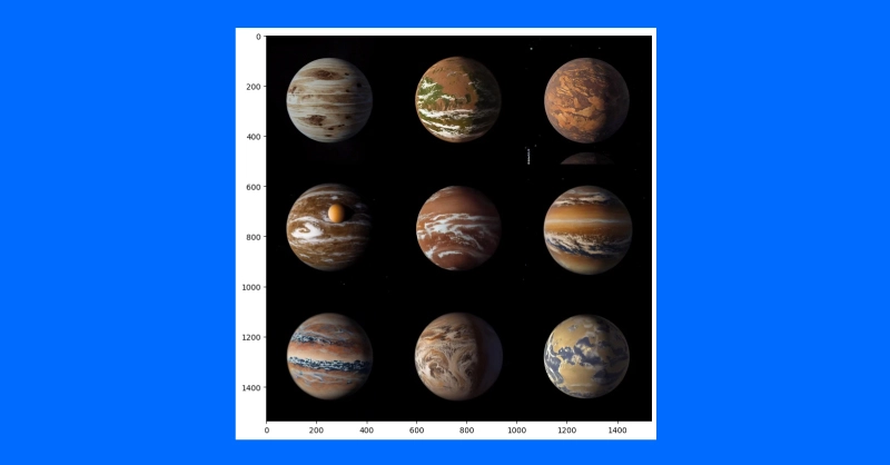
By feeding the model an example initial image, we can generate similar images. You can also use a text-guided image-to-image pipeline to change the style of an image by increasing the guidance, adding negative prompts and more such as “non-realistic” or “watercolor” or “paper sketch.” Your mile may vary and adjusting your prompts will be the easiest way to find the right image you want to create.
Despite the discourse behind diffusion systems and imitating human generated art, diffusion models have other more impactful purposes. It has been applied to protein folding prediction for protein design and drug development. Text-to-video is also an active area of research and is offered by several companies (e.g. Stability AI, Google). Diffusion is also an emerging approach for text-to-speech applications.
It’s clear that the diffusion process is taking a central role in the evolution of AI and the interaction of technology with the global human environment. While the intricacies of copyright, other intellectual property laws, and the impact on human art and science are evident in both positive and negative ways. But what is truly a positive is the unprecedented capability AI has to understand language and generate images. It was AlexNet that had computers analyze an image and output text, and only now computers can analyze textual prompts and output coherent images.

Training AI models on massive datasets can be accelerated exponentially with the right system. It's not just a high-performance computer, but a tool to propel and accelerate your research.
Configure NowDenoising diffusion models are trained to pull patterns out of noise, to generate a desirable image. The training process involves showing model examples of images (or other data) with varying levels of noise determined according to a noise scheduling algorithm, intending to predict what parts of the data are noise. If successful, the noise prediction model will be able to gradually build up a realistic-looking image from pure noise, subtracting increments of noise from the image at each time step.
Unlike the image at the top of this section, modern diffusion models don’t predict noise from an image with added noise, at least not directly. Instead, they predict noise in a latent space representation of the image. Latent space represents images in a compressed set of numerical features, the output of an encoding module from a variational autoencoder, or VAE. This trick put the “latent” in latent diffusion, and greatly reduced the time and computational requirements for generating images. As reported by the paper authors, latent diffusion speeds up inference by at least ~2.7X over direct diffusion and trains about three times faster.
People working with latent diffusion often talk of using a “diffusion model,” but in fact, the diffusion process employs several modules. As in the diagram above, a diffusion pipeline for text-to-image workflows typically includes a text embedding model (and its tokenizer), a denoise prediction/diffusion model, and an image decoder. Another important part of latent diffusion is the scheduler, which determines how the noise is scaled and updated over a series of “time steps” (a series of iterative updates that gradually remove noise from latent space).
We’ll use CompVis/latent-diffusion-v1-4 for most of our examples. Text embedding is handled by a CLIPTextModel and CLIPTokenizer. Noise prediction uses a ‘U-Net,’ a type of image-to-image model that originally gained traction as a model for applications in biomedical images (especially segmentation). To generate images from denoised latent arrays, the pipeline uses a variational autoencoder (VAE) for image decoding, turning those arrays into images.
We’ll start by building our version of this pipeline from HuggingFace components.
# local setup
virtualenv diff_env –python=python3.8
source diff_env/bin/activate
pip install diffusers transformers huggingface-hub
pip install torch --index-url https://download.pytorch.org/whl/cu118
Make sure to check pytorch.org to ensure the right version for your system if you’re working locally. Our imports are relatively straightforward, and the code snippet below suffices for all the following demos.
import os
import numpy as np
import torch
from diffusers import StableDiffusionPipeline, AutoPipelineForImage2Image
from diffusers.pipelines.pipeline_utils import numpy_to_pil
from transformers import CLIPTokenizer, CLIPTextModel
from diffusers import AutoencoderKL, UNet2DConditionModel, \
       PNDMScheduler, LMSDiscreteScheduler

from PIL import Image
import matplotlib.pyplot as plt
Now for the details. Start by defining image and diffusion parameters and a prompt.
prompt = [" "]

# image settings
height, width = 512, 512

# diffusion settings
number_inference_steps = 64
guidance_scale = 9.0
batch_size = 1
Initialize your pseudorandom number generator with a seed of your choice for reproducing your results.
def seed_all(seed):
    torch.manual_seed(seed)
    np.random.seed(seed)

seed_all(193)
Now we can initialize the text embedding model, autoencoder, a U-Net, and the time step scheduler.
tokenizer = CLIPTokenizer.from_pretrained("openai/clip-vit-large-patch14")
text_encoder = CLIPTextModel.from_pretrained("openai/clip-vit-large-patch14")
vae = AutoencoderKL.from_pretrained("CompVis/stable-diffusion-v1-4", \
        subfolder="vae")
unet = UNet2DConditionModel.from_pretrained("CompVis/stable-diffusion-v1-4",\
        subfolder="unet")
scheduler = PNDMScheduler()
scheduler.set_timesteps(number_inference_steps)

my_device = torch.device("cuda") if torch.cuda.is_available() else torch.device("cpu")
vae = vae.to(my_device)
text_encoder = text_encoder.to(my_device)
unet = unet.to(my_device)
Encoding the text prompt as an embedding requires first tokenizing the string input. Tokenization replaces characters with integer codes corresponding to a vocabulary of semantic units, e.g. via byte pair encoding (BPE). Our pipeline embeds a null prompt (no text) alongside the textual prompt for our image. This balances the diffusion process between the provided description and natural-appearing images in general. We’ll see how to change the relative weighting of these components later in this article.
prompt = prompt * batch_size
tokens = tokenizer(prompt, padding="max_length",\
max_length=tokenizer.model_max_length, truncation=True,\
        return_tensors="pt")

empty_tokens = tokenizer([""] * batch_size, padding="max_length",\
max_length=tokenizer.model_max_length, truncation=True,\
        return_tensors="pt")


with torch.no_grad():
    text_embeddings = text_encoder(tokens.input_ids.to(my_device))[0]
    max_length = tokens.input_ids.shape[-1]
    notext_embeddings = text_encoder(empty_tokens.input_ids.to(my_device))[0]
    text_embeddings = torch.cat([notext_embeddings, text_embeddings])
We initialize latent space as random normal noise and scale it according to our diffusion time step scheduler.
latents = torch.randn(batch_size, unet.config.in_channels, \
        height//8, width//8)
latents = (latents * scheduler.init_noise_sigma).to(my_device)
Everything is ready to go, and we can dive into the diffusion loop itself. We can keep track of images by sampling periodically throughout so we can see how noise is gradually decreased.
images = []
display_every = number_inference_steps // 8

# diffusion loop
for step_idx, timestep in enumerate(scheduler.timesteps):
    with torch.no_grad():
        # concatenate latents, to run null/text prompt in parallel.
        model_in = torch.cat([latents] * 2)
        model_in = scheduler.scale_model_input(model_in,\
                timestep).to(my_device)
        predicted_noise = unet(model_in, timestep, \
                encoder_hidden_states=text_embeddings).sample
        # pnu - empty prompt unconditioned noise prediction
        # pnc - text prompt conditioned noise prediction
        pnu, pnc = predicted_noise.chunk(2)
        # weight noise predictions according to guidance scale
        predicted_noise = pnu + guidance_scale * (pnc - pnu)
        # update the latents
        latents = scheduler.step(predicted_noise, \
                timestep, latents).prev_sample
        # Periodically log images and print progress during diffusion
        if step_idx % display_every == 0\
                or step_idx + 1 == len(scheduler.timesteps):
           image = vae.decode(latents / 0.18215).sample[0]
           image = ((image / 2.) + 0.5).cpu().permute(1,2,0).numpy()
           image = np.clip(image, 0, 1.0)
           images.extend(numpy_to_pil(image))
           print(f"step {step_idx}/{number_inference_steps}: {timestep:.4f}")
At the end of the diffusion process, we have a decent rendering of what you wanted to generate. Next, we’ll go over additional techniques for greater control. As we’ve already made our diffusion pipeline, we can use the streamlined diffusion pipeline from HuggingFace for the rest of our examples.
With the latest CPUs and most powerful GPUs available, accelerate your deep learning and AI project optimized to your deployment, budget, and desired performance!
Configure NowWe’ll use a set of helper functions in this section:
def seed_all(seed):
    torch.manual_seed(seed)
    np.random.seed(seed)

def grid_show(images, rows=3):
    number_images = len(images)
    height, width = images[0].size
    columns = int(np.ceil(number_images / rows))
    grid = np.zeros((height*rows,width*columns,3))
    for ii, image in enumerate(images):
        grid[ii//columns*height:ii//columns*height+height, \
                ii%columns*width:ii%columns*width+width] = image
        fig, ax = plt.subplots(1,1, figsize=(3*columns, 3*rows))
        ax.imshow(grid / grid.max())
    return grid, fig, ax

def callback_stash_latents(ii, tt, latents):
    # adapted from fastai/diffusion-nbs/stable_diffusion.ipynb
    latents = 1.0 / 0.18215 * latents
    image = pipe.vae.decode(latents).sample[0]
    image = (image / 2. + 0.5).cpu().permute(1,2,0).numpy()
    image = np.clip(image, 0, 1.0)
    images.extend(pipe.numpy_to_pil(image))

my_seed = 193
We’ll start with the most well-known and straightforward application of diffusion models: image generation from textual prompts, known as text-to-image generation. The model we’ll use was released into the wild (of the Hugging Face Hub) by the academic lab that published the latent diffusion paper. Hugging Face coordinates workflows like latent diffusion via the convenient pipeline API. We want to define what device and what floating point to calculate based on if we have or do not have a GPU.
if (1):
    #Run CompVis/stable-diffusion-v1-4 on GPU
    pipe_name = "CompVis/stable-diffusion-v1-4"
    my_dtype = torch.float16
    my_device = torch.device("cuda")
    my_variant = "fp16"
    pipe = StableDiffusionPipeline.from_pretrained(pipe_name,\
    safety_checker=None, variant=my_variant,\
        torch_dtype=my_dtype).to(my_device)
else:
    #Run CompVis/stable-diffusion-v1-4 on CPU
    pipe_name = "CompVis/stable-diffusion-v1-4"
    my_dtype = torch.float32
    my_device = torch.device("cpu")
    pipe = StableDiffusionPipeline.from_pretrained(pipe_name, \
            torch_dtype=my_dtype).to(my_device)
If you use a very unusual text prompt (very unlike those in the dataset), it’s possible to end up in a less-traveled part of latent space. The null prompt embedding provides a balance and combining the two according to guidance_scale allows you to trade off the specificity of your prompt against common image characteristics.
guidance_images = []
for guidance in [0.25, 0.5, 1.0, 2.0, 4.0, 6.0, 8.0, 10.0, 20.0]:
    seed_all(my_seed)
    my_output = pipe(my_prompt, num_inference_steps=50, \
    num_images_per_prompt=1, guidance_scale=guidance)
    guidance_images.append(my_output.images[0])
    for ii, img in enumerate(my_output.images):
        img.save(f"prompt_{my_seed}_g{int(guidance*2)}_{ii}.jpg")

temp = grid_show(guidance_images, rows=3)
plt.savefig("prompt_guidance.jpg")
plt.show()
Since we generated the prompt using the 9 guidance coefficients, you can plot the prompt and view how the diffusion developed. The default guidance coefficient is 0.75 so on the 7th image would be the default image output.
Sometimes latent diffusion really “wants” to produce an image that doesn’t match your intentions. In these scenarios, you can use a negative prompt to push the diffusion process away from undesirable outputs. For example, we could use a negative prompt to make our Martian astronaut diffusion outputs a little less human.
my_prompt = " "
my_negative_prompt = " "

output_x = pipe(my_prompt, num_inference_steps=50, num_images_per_prompt=9, \
        negative_prompt=my_negative_prompt)

temp = grid_show(output_x)
plt.show()
You should receive outputs that follow your prompt while avoiding outputting the things described in your negative prompt.
Text-to-image generation from scratch is not the only application for diffusion pipelines. Actually, diffusion is well-suited for image modification, starting from an initial image. We’ll use a slightly different pipeline and pre-trained model tuned for image-to-image diffusion.
pipe_img2img = AutoPipelineForImage2Image.from_pretrained(\

        "runwayml/stable-diffusion-v1-5", safety_checker=None,\

torch_dtype=my_dtype, use_safetensors=True).to(my_device)
One application of this approach is to generate variations on a theme. A concept artist might use this technique to quickly iterate different ideas for illustrating an exoplanet based on the latest research.
We’ll first download a public domain artist’s concept of planet 1e in the TRAPPIST system (credit: NASA/JPL-Caltech). Then, after downscaling to remove details, we’ll use a diffusion pipeline to make several different versions of the exoplanet TRAPPIST-1e.
url = \
"https://upload.wikimedia.org/wikipedia/commons/thumb/3/38/TRAPPIST-1e_artist_impression_2018.png/600px-TRAPPIST-1e_artist_impression_2018.png"
img_path = url.split("/")[-1]
if not (os.path.exists("600px-TRAPPIST-1e_artist_impression_2018.png")):
    os.system(f"wget \     '{url}'")
    init_image = Image.open(img_path)

seed_all(my_seed)

trappist_prompt = "Artist's impression of TRAPPIST-1e"\
                  "large Earth-like water-world exoplanet with oceans,"\
                  "NASA, artist concept, realistic, detailed, intricate"

my_negative_prompt = "cartoon, sketch, orbiting moon"

my_output_trappist1e = pipe_img2img(prompt=trappist_prompt, num_images_per_prompt=9, \
     image=init_image, negative_prompt=my_negative_prompt, guidance_scale=6.0)

grid_show(my_output_trappist1e.images)
plt.show()
By feeding the model an example initial image, we can generate similar images. You can also use a text-guided image-to-image pipeline to change the style of an image by increasing the guidance, adding negative prompts and more such as “non-realistic” or “watercolor” or “paper sketch.” Your mile may vary and adjusting your prompts will be the easiest way to find the right image you want to create.
Despite the discourse behind diffusion systems and imitating human generated art, diffusion models have other more impactful purposes. It has been applied to protein folding prediction for protein design and drug development. Text-to-video is also an active area of research and is offered by several companies (e.g. Stability AI, Google). Diffusion is also an emerging approach for text-to-speech applications.
It’s clear that the diffusion process is taking a central role in the evolution of AI and the interaction of technology with the global human environment. While the intricacies of copyright, other intellectual property laws, and the impact on human art and science are evident in both positive and negative ways. But what is truly a positive is the unprecedented capability AI has to understand language and generate images. It was AlexNet that had computers analyze an image and output text, and only now computers can analyze textual prompts and output coherent images.
Training AI models on massive datasets can be accelerated exponentially with the right system. It's not just a high-performance computer, but a tool to propel and accelerate your research.
Configure Now